Science

Maximum Likelihood Estimation

This is my 1000th post. While the likelihood of reaching post # 1000 in as many days is one topic for a future post, today we specifically develop some intuition around MLE or the maximum likelihood estimate.

A coin lands H, H, T, T, H. How likely is this to happen? A simplistic way is to think that this coin always lands in this pattern (H, H, T, T, H). We know that is not credible. Let’s assign the coin a probability p (“the parameter”) to land heads. So, the question we want to answer is: at what probability (of occurrence for heads), p, does the likelihood maximise?

Step 1: What is the probability of observing the sequence HHTTH? Let’s assume all flips are independent. The probability is
p x p x (1-p) x (1-p) x p = p3 x (1-p)2

Step 2: What is the value of p at which the likelihood of observing HHTTH is maximised? We will take help from calculus, take a derivative, equate to zero, and solve for p.

3p2 x (1-p)2 – 2 p3 x (1-p) = 0
3(1-p) – 2p = 0
p = 3/5 = 0.6

Ok, the MLE for this sequence is 0.6. But what is the probability of the sequence happening? For that, substitute the value of p in the equation,
0.6 x 0.6 x (1-0.6) x (1-0.6) x 0.6 = 0.03456

Conclusion: if the coin lands on heads 60% of the time, the probability of seeing the sequence HHTTH is 3.456%. 3.456% may appear small, but it is better than any other p.
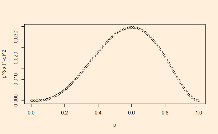
Continuous distribution

If a person’s height is 66 inches, which population is she from? It is unusually rare that a region has only people 66 inches tall. We assume that people’s heights follow a normal distribution with a standard deviation (say, 4). So, the question becomes: What is the most likely distribution that person is from?
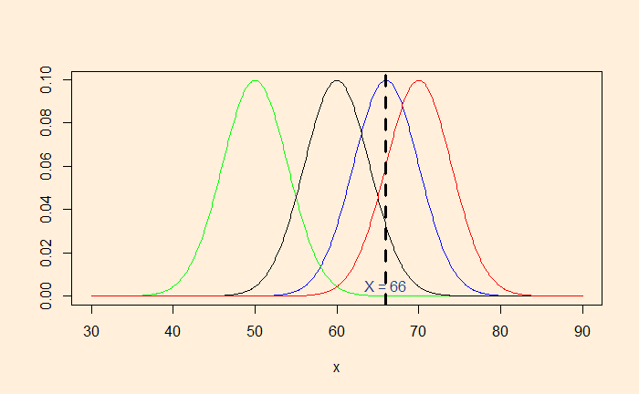
Here are a few distributions with the standard deviation 4. By placing a market at x = 66, you can observe that the distribution with mean = 66 is the most likely (the highest point) to represent the observed data.

Instead, we collected two data, 66 and 58 inches. The blue curve strongly supports 66, but not much 58. MLE will balance the probabilities so that it can include both the data.
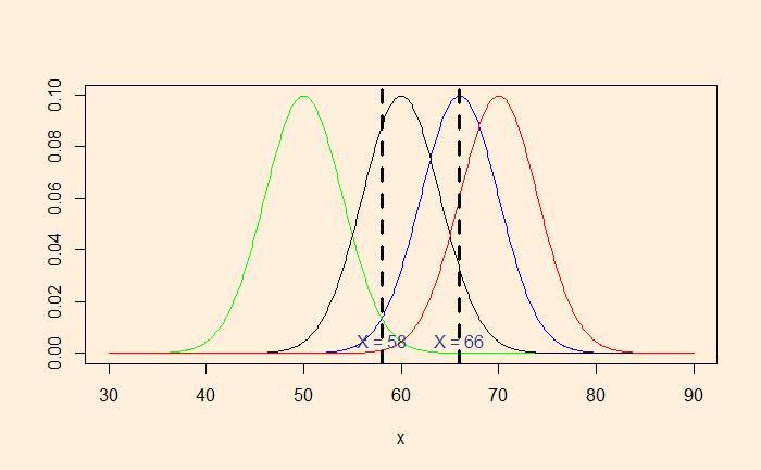
The average of 66 and 58 (= 62) will maximise the likelihood.

Reference

Maximum Likelihood Estimation: Brian Greco – Learn Statistics

Maximum Likelihood Estimation Read More »

Employee Attrition Dataset

We continue using the ‘tigerstats’ package to analyse the ‘IBM HR Analytics Employee Attrition & Performance’ dataset, a fictional data set created by IBM data scientists and taken from Kaggle. The dataset contains various parameters related to attribution,

Em_data <- read.csv("D:/04Compute/Web/Employee-Attrition.csv")
str(Em_data)
'data.frame':	1470 obs. of  35 variables:
 $ Age                     : int  41 49 37 33 27 32 59 30 38 36 ...
 $ Attrition               : chr  "Yes" "No" "Yes" "No" ...
 $ BusinessTravel          : chr  "Travel_Rarely" "Travel_Frequently" "Travel_Rarely" "Travel_Frequently" ...
 $ DailyRate               : int  1102 279 1373 1392 591 1005 1324 1358 216 1299 ...
 $ Department              : chr  "Sales" "Research & Development" "Research & Development" "Research & Development" ...
 $ DistanceFromHome        : int  1 8 2 3 2 2 3 24 23 27 ...
 $ Education               : int  2 1 2 4 1 2 3 1 3 3 ...
 $ EducationField          : chr  "Life Sciences" "Life Sciences" "Other" "Life Sciences" ...
 $ EmployeeCount           : int  1 1 1 1 1 1 1 1 1 1 ...
 $ EmployeeNumber          : int  1 2 4 5 7 8 10 11 12 13 ...
 $ EnvironmentSatisfaction : int  2 3 4 4 1 4 3 4 4 3 ...
 $ Gender                  : chr  "Female" "Male" "Male" "Female" ...
 $ HourlyRate              : int  94 61 92 56 40 79 81 67 44 94 ...
 $ JobInvolvement          : int  3 2 2 3 3 3 4 3 2 3 ...
 $ JobLevel                : int  2 2 1 1 1 1 1 1 3 2 ...
 $ JobRole                 : chr  "Sales Executive" "Research Scientist" "Laboratory Technician" "Research Scientist" ...
 $ JobSatisfaction         : int  4 2 3 3 2 4 1 3 3 3 ...
 $ MaritalStatus           : chr  "Single" "Married" "Single" "Married" ...
 $ MonthlyIncome           : int  5993 5130 2090 2909 3468 3068 2670 2693 9526 5237 ...
 $ MonthlyRate             : int  19479 24907 2396 23159 16632 11864 9964 13335 8787 16577 ...
 $ NumCompaniesWorked      : int  8 1 6 1 9 0 4 1 0 6 ...
 $ Over18                  : chr  "Y" "Y" "Y" "Y" ...
 $ OverTime                : chr  "Yes" "No" "Yes" "Yes" ...
 $ PercentSalaryHike       : int  11 23 15 11 12 13 20 22 21 13 ...
 $ PerformanceRating       : int  3 4 3 3 3 3 4 4 4 3 ...
 $ RelationshipSatisfaction: int  1 4 2 3 4 3 1 2 2 2 ...
 $ StandardHours           : int  80 80 80 80 80 80 80 80 80 80 ...
 $ StockOptionLevel        : int  0 1 0 0 1 0 3 1 0 2 ...
 $ TotalWorkingYears       : int  8 10 7 8 6 8 12 1 10 17 ...
 $ TrainingTimesLastYear   : int  0 3 3 3 3 2 3 2 2 3 ...
 $ WorkLifeBalance         : int  1 3 3 3 3 2 2 3 3 2 ...
 $ YearsAtCompany          : int  6 10 0 8 2 7 1 1 9 7 ...
 $ YearsInCurrentRole      : int  4 7 0 7 2 7 0 0 7 7 ...
 $ YearsSinceLastPromotion : int  0 1 0 3 2 3 0 0 1 7 ...
 $ YearsWithCurrManager    : int  5 7 0 0 2 6 0 0 8 7 ...

barchartGC

barchartGC(~Gender,data=Em_data)
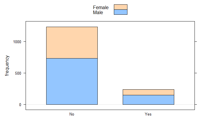
barchartGC(~Attrition+Gender,data=Em_data, stack = TRUE)

xtabs

xtabs(~Attrition+MaritalStatus,data=Em_data)
         MaritalStatus
Attrition Divorced Married Single
      No       294     589    350
      Yes       33      84    120
xtabs(~Attrition+Gender,data=Em_data)
         Gender
Attrition Female Male
      No     501  732
      Yes     87  150

CIMean

CIMean(~MonthlyIncome,data=Em_data)

ttestGC

ttestGC(~MonthlyIncome,data=Em_data)
Inferential Procedures for One Mean mu:

Descriptive Results:

variable       mean     sd       n          
MonthlyIncome  6502.931 4707.957 1470       

Inferential Results:

Estimate of mu:	 6503 
SE(x.bar):	 122.8 

95% Confidence Interval for mu:

          lower.bound         upper.bound          
          6262.062872         6743.799713      
ttestGC(~Age,data=Em_data)
Inferential Procedures for One Mean mu:

Descriptive Results:

variable  mean     sd       n          
Age       36.924   9.135    1470       

Inferential Results:

Estimate of mu:	 36.92 
SE(x.bar):	 0.2383 

95% Confidence Interval for mu:

          lower.bound         upper.bound          
          36.456426           37.391193 

Employee Attrition Dataset Read More »

Goodness of Fit using tigerstats

We have seen how the R package ‘tigerstats’ can help visualise basic statistics. The library has several functions and datasets to teach statistics at an elementary level. We will see a couple of them that enable hypothesis testing.

chi-square test

We start with a test for Independence using the chi-square test. The example is the same as we used previously. Here, we create the database with the following summary.

High SchoolBachelorsMastersPh.d.Total
Female60544641201
Male40445357194
Total100989998395
as_tibble(educ)

The function to use is ‘chisqtestGC’, which takes two variables (~var1 + var2) to test their association. Additional attributes such as graph and verbose yield the relevant graph (ch-square curve) for the P-value and details of the output.

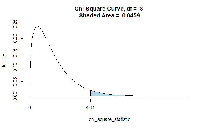
chisqtestGC(~EDU+SEX, data=educ, graph = TRUE, verbose = TRUE)
Pearson's Chi-squared test 

Observed Counts:
             SEX
EDU           Female Male
  Bachelors       54   44
  High School     60   40
  Masters         46   53
  Ph.d.           41   57

Counts Expected by Null:
             SEX
EDU           Female  Male
  Bachelors    49.87 48.13
  High School  50.89 49.11
  Masters      50.38 48.62
  Ph.d.        49.87 48.13

Contributions to the chi-square statistic:
             SEX
EDU           Female Male
  Bachelors     0.34 0.35
  High School   1.63 1.69
  Masters       0.38 0.39
  Ph.d.         1.58 1.63


Chi-Square Statistic = 8.0061 
Degrees of Freedom of the table = 3 
P-Value = 0.0459 

Binomial test for proportion

Suppose a coin toss landed on 40 heads in 100 attempts. Perform a two-sided hypothesis test for p = 0.5 as the Null.

binomtestGC(x=40,n=100,p=0.5, alternative = "two.sided", graph = TRUE, conf.level = 0.95)

x = variable under study
n = size of the sample
p = Null Hypothesis value for population proportion
alternative = takes “two.sided”, “less” or “greater” for the computation of the p-value.
conf.level = number between 0 and 1, indicating the confidence interval
graph = If TRUE, plot graph of p-value

Exact Binomial Procedures for a Single Proportion p:
	Results based on Summary Data

Descriptive Results:  40 successes in 100 trials

Inferential Results:

Estimate of p:	 0.4 
SE(p.hat):	 0.049 

95% Confidence Interval for p:

          lower.bound         upper.bound          
          0.303295            0.502791             

Test of Significance:

	H_0:  p = 0.5 
	H_a:  p != 0.5 

	P-value:		P = 0.0569 
binomtestGC(x=40,n=100,p=0.5, alternative = "less", graph = TRUE, conf.level = 0.95)
Exact Binomial Procedures for a Single Proportion p:
	Results based on Summary Data

Descriptive Results:  40 successes in 100 trials

Inferential Results:

Estimate of p:	 0.4 
SE(p.hat):	 0.049 

95% Confidence Interval for p:

          lower.bound         upper.bound          
          0.000000            0.487024             

Test of Significance:

	H_0:  p = 0.5 
	H_a:  p < 0.5 

	P-value:		P = 0.0284 

Goodness of Fit using tigerstats Read More »

Probability, Likelihood and tigerstats

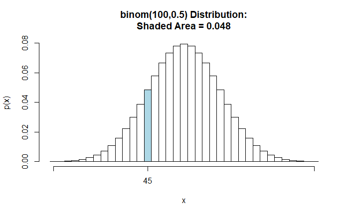
This post refreshes the probability vs likelihood concept and presents a few R functions from the tigerstats library. As usual, we begin with a coin-flipping exercise. What is the probability of obtaining 45 heads upon flipping 100 fair coins? A fair coin is one in which the chance of getting heads equals the chance of getting tails: 0.5.

Here is a graphical representation of the ask.

library(tigerstats)
bound <- c(45,45)
pbinomGC(bound,region="between",size=100,prob=0.5,graph=TRUE)

Coin tossing is a discrete event, and the Y-axis represents the probability. The probability of obtaining 45 heads while flipping 100 fair coins is 0.048.

Now, consider a continuous distribution. Suppose the heights of adults are normally distributed in a population with a mean of 175 cm and a standard deviation of 6.5 cm. What is the probability that a random person measures height between 185 and 190 cm?

sample <- c(185,190)
pnormGC(bound=sample,region="between", mean=175,sd=6.5,graph=TRUE)

Notice a few things: the Y-axis is not probability but probability density. The required probability is the area (under the curve) between two values, the height between 185 and 190 cm = 0.0515. In a continuous distribution, where the probability can take every possible value between 0 and 1, getting the chance for precise height (say, 180.0000) does not make sense.

Likelihood

If probability was about getting 45 heads for a coin with p = 0.5 tossed 100 times, the likelihood is the mirror image of that. What is the likelihood of having a fair coin (p = 0.5) if the coin lands 45 heads in 100 tosses?

In likelihood discussions, you have the data, i.e., 45 heads in 100 tosses. The investigator’s task is to find out the coin bias.
The likelihood that it’s an unbiased coin (p = 0.5), given that 45 in 100 landed on heads, is 0.048.
The likelihood that the coin is biased with p = 0.55, given that 45 in 100 landed on heads, is 0.011.
The likelihood that the coin is biased p = 0.4, given that 45 in 100 landed on heads, is 0.048.

Similarly, for heights,
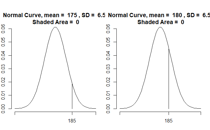
The likelihood of a distribution with mean = 175 cm and a standard deviation = 6.5 cm, given the measured height = 185, is 0.019
The likelihood of a distribution with mean = 180 cm and a standard deviation = 6.5 cm, given the measured height = 185, is 0.046

In summary

Probability is about the chance of data under a given distribution, P(Data|Distribution)

Likelihood is about the distribution for the given data, L(Distribution|Data)

Reference

Probability is not Likelihood. Find out why!!!: StatQuest with Josh Starmer

Probability, Likelihood and tigerstats Read More »

Drug Development and the Valley of Death

One of the biggest beneficiaries of scientific methodology is evidence-based modern medicine. Each step in the ‘bench to bedside‘ process is a testimony of the scientific rigour in medicine research. While the low probability of success (PoS) at each stage is a challenge in the race to fight against diseases, it increases the confidence level in the validity of the final product.

The drug development process is divided into two parts: basic research and clinical research. Translational research is the bridge that connects the two parts. The ‘T Spectrum’ consists of 5 stages,

T0 includes preclinical and animal studies.
T1 is the phase 1 clinical trial for safety and proof of concept
T2 is the phase 2/3 clinical trial for efficacy and safety
T3 includes the phase 4 clinical trial towards clinical outcome and
T4 leads to approval for usage by communities.

Probability of success

According to a publication by Seyhan, who quotes NIH, 80 to 90% of research projects fail before the clinical stage. The following are typical rates of success in clinical drug development stages:
Phase 1 to Phase 2: 52%
Phase 2 to Phase 3: 28.9%
Phase 3 to Phase 4: 57.8%
Phase 4 to approval: 90.6%
The data used to arrive at the above statistics was collected from 12,728 clinical and regulatory phase transitions of 9,704 development programs across 1,779 companies in the Biomedtracker database between 2011 and 2020.

The overall chance of success from lab to shop thus becomes:
0.1×0.52×0.289×0.578×0.906 = 0.008 or < 1%!

References

Seyhan, A. A.; Translational Medicine Communications, 2019, 4-18
Mohsa, R.C.; Greig, N. H.; Alzheimer’s & Dementia: Translational Research & Clinical Interventions 3, 2017, 651-657
Cummings, J.L.; Morstorf, T.; Zhong, K.; Alzheimer’s Research & Therapy, 2014, 6-37
Paul, S.M; Mytelka, D.S.; Dunwiddie, C. T.; Persinger, C. C.; Munos, B.H.; Lindborg, S.R.; Schacht, A. L, Nature Reviews – Drug Discovery, 2010, VOlume 9.
What is Translational Research?: UAMS

Drug Development and the Valley of Death Read More »

Hardy-Weinberg – Applied

Here is a problem to illustrate how the Hardy-Weinberg Principle is applied.

In a population of 130,000 special mice, green fur is dominant over orange. If there are 300 orange mice in the population of 130,000, find the following:
Frequency of green allele
Frequency of orange allele
Frequency of each genotype

p + q = 1
p2 + 2 pq + q2 = 1

We must start with orange as it is the recessive one. It is because, from the dominant (green) colour, it is impossible to say that it is homozygous dominant or heterozygous. Whereas only homozygous recessive has orange fur.

q2 = 300/130,000 = 0.0023
q = sqrt(q2) = 0.048
p = 1 – q = 0.95

Genotype Frequencies:
homozygous dominant = p2 = 0.90
Heterozygous = 2pq = 0.0456 = 0.091
Homozygous recessive = q2 = 0.0023

Reference

The Hardy-Weinberg Principle: Watch your Ps and Qs: ThePenguinProf

Hardy-Weinberg – Applied Read More »

Hardy-Weinberg – Continued

We have seen the terms allele, dominant, recessive, genotype, phenotype, etc. Consider a population with five individuals with the following gene pairs. Assume they dictate the hair colour. So, the red gene is for red hair colour and black for black. But red is recessive, and black is dominant. That means.

red-red = red hair
red-black = black hair
black-black = black hair

So we have two people with red hair (homozygous recessive) and three with black hair (two heterozygous and one homozygous dominant).

Hardy Weinberg rule

The rule states that allele and genotype frequencies in a population will remain constant in the absence of other evolutionary processes such as migration, mutation, selection, etc.

To estimate the allele frequency, we create the gene pool, the aggregate of all alleles of the population. Our gene pool has ten alleles, with six reds and four blacks.

Let p represent the allele frequency of the dominant trait and q that of the recessive.
p = 4/10 = 0.4
q = 6/10 = 0.6
p + q = constant = 1

To estimate genotype frequency, consider the following. If we take one random gene from the pool, what is the probability that it is red? It will be q. What is the chance of picking two genes to form a homozygous recessive? It will be q x q = q2. Similarly, to pull out a black followed by another black is p2 and a black and a red is 2pq (black followed by red OR red followed by black; add them because of OR rule).

The genotype frequency is the sum of those three types, i.e., p2 + 2 pq + q2. Needless to say, that will be 1. To summarise, the following are the two governing equations.

p + q = 1
p2 + 2 pq + q2 = 1

Hardy-Weinberg – Continued Read More »

Hardy-Weinberg Principle

We have two copies of every gene; each copy is called an allele. If both copies of alleles are the same, it’s homozygous. On the other hand, if they are different, it’s heterozygous. The terms dominant and recessive mean two different inheritance patterns of traits.

Imagine hair colour as a trait. The dominant is black, and the recessive is red. Note this doesn’t mean black hair dominates or anything like that. It only means:

black allele + black allele = black trait
black allele + red allele = black trait
red allele + red allele = red trait

Simply put, you need both the recessive alleles to get a recessive trait, whereas one dominant allele is sufficient to get the dominant trait.

Also, the allele pairs (black, black), (black, red) and (red, red) are all genotypes. On the other hand, the traits – black hair and red hair are two phenotypes. If a genotype is what your genes are, then a phenotype is what you look like!

Before Hardy and Weinberg, people used to get puzzled by the fact that the population did not end up having only the dominant traits. Their principle (developed independently) states that frequencies of alleles and genotypes in a population will remain constant over time in the absence of other evolutionary influences.

Hardy-Weinberg Principle Read More »

Chance of DMD

A woman who has a family history of Duchenne muscular dystrophy (DMD) gets tested for the presence of disease using a test (creatine phosphokinase, CPK) that has a sensitivity of 67% and a specificity of 95%. It is known that her brother has the condition. What is the probability that she is a carrier of the condition, and further, what is the chance that her son will have the disease if she tests negative in the CPK?

The conditional probability of disease, given the negative test result. We will use Bayes’ theorem to estimate the probability.

P(C|-ve) = \frac{P(-ve|C) P(C)}{P(-ve|C) P(C) + P(-ve|nC) P(nC)}

P(C|-ve) denotes the probability that she is a carrier (C), given she tested negative for the conditions (-ve).

P(-ve|C) is the chance of a negative result, given the person is a carrier. We know the chance of a +ve results if the person carries the gene. It is the sensitivity and is 67%. This means if the person carries a gene, there is a 67% chance of getting a positive and a 33% chance of getting a negative result. Therefore, P(-ve|C) = 0.33.

P(-ve|nC) is the chance of a negative result, given the person is NOT a carrier. It is nothing but specificity, and it is 95%. Therefore, P(-ve|nC) = 0.95.

This leaves the final two parameters: the prior probabilities that she carries or does not carry the disease genes (P(C) and P(nC)). DMD happens because of a mutated gene on the X chromosome. In our case, the woman can get that X chromosome from her father or mother. Since her brother had the conditions, and he could get X only from his mother, the mother is certainly a carrier of the mutated gene. Since the daughter inherited one of two Xs from her mother, P(C) = 0.5, which means P(nC) is 0.5.

Applying the Bayes’ theorem,

P(C|-ve) = \frac{0.33*0.5}{0.33*0.5 + 0.95*0.5} = 0.26

If she is a carrier (there is a 26% chance), she could pass one of her X chromosomes to her son at a 50% chance. This implies that the probability that her son gets the disease is 0.26 x 0.5 = 0.13 or 13%.

Reference

Bayesian Analysis and Risk Assessment in Genetic Counseling and Testing: Journal of Molecular Diagnostics, Vol. 6, No. 1, February 2004

Chance of DMD Read More »

The Advanced One

Which is the most advanced form of life?

Before we reach the answer, we must know that evolution is not a linear process (like a ladder), unlike what Aristotle thought, but a branched (like a tree). Consider the family of Apes. The apes (Hominoidea) branches into two families – the ‘great apes’ and the ‘lesser apes’.

The lesser apes contain a bunch of gibbons. The great apes are further divided into two – Homininae and orangutans.

Does this picture mean the orangutans and homininae are higher than the gibbons? No, and the scheme can also be drawn in the following way.

Homininae goes to gorillas and hominini. In other words, the gorillas and the hominini have a common ancestor. Hominini then goes to pan (chimpanzees and bonobos) and humans.

You may conclude that an advanced species goes from left to right. That is also not true. The picture can also be like this.

All these living lineages have the same amount of time to evolve; therefore, they are equal!

Reference

Ape: Wiki

Understanding Evolution: Berkeley

The Advanced One Read More »