Life

Monthly Miracle

During the time that we are awake and actively engaged in living our lives, roughly for eight hour each day, we see and hear things happening at a rate of about one per second. So the total number of events that happen to us is about thirty thousand per day, or about a million per month. With few exceptions, these events are not miracles because they are insignificant. The chance of a miracle is about one per million events. Therefore we should expect about one miracle to happen, on the average, every month

Freeman Dyson

Morgan Housel’s latest book, Same as Ever’, continues from where he left off in his earlier very popular, “The Psychology of Money”. It’s about human psychology and its inability to comprehend probability.

The brain always craves certainty or a black-or-white world. And even trained people find it challenging to reconcile with the math behind chances. The lottery winning odds, as perceived by journalists in the last post, is just one example of that. The result is that newspapers continue to display shocking headlines, reinforcing people’s trust in magic and divine interventions.

Here is an example: in a world with 8 billion humans, how many rarest of rare events, i.e., something with a probability of occurrence of once in a billion in a year, happens in a year? It seems difficult to imagine 8 billion people interacting with their surroundings is analogous to 8 billion independent binomial trials:

P(s; p, n) = nCs x ps (1-p)n-s

The formula represents the probability of s number of ‘success’ if n number of independent trials happen, each with a chance of p. In our problem, substitute n with 8 billion and p with 1/1,000,000,000.

The probability of no ‘miracle’ happening in a year, i.e., s = 0.

P(0; 1×10⁻⁹, 8×10⁹) = 1 x 1 x (1-1×10⁻⁹)8e9

The answer is almost ZERO; subtracting 10-9 from 1 gives a fraction just short of 1, which multiplies by itself a few billion times, and the answer leads to nearly nothing.

You can evaluate the formula for s = 1, 2, etc. We will use the R function for that and plot.

s <- seq(0,15)
plot(s, dbinom(s, 8e9, 1e-9))

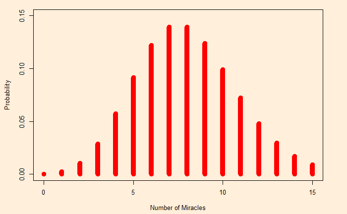
There is more than a 10% chance to see 5, 6, 7, 8, 9 or 10 miracles in a given year. The only thing is: it can’t say where it will happen; it will happen somewhere, and the journalist will dig it up to her headlines.

Monthly Miracle Read More »

Weibull and Rayleigh Distributions

We have seen Weibull before. It is a continuous probability distribution that finds applications in various fields, such as engineering and reliability analysis. It is because of the flexibility to adapt to different shapes: uniform, left, or right-skew.

The shape and scale are the names of two typical parameters in a Weibull distribution. Depending on their values, one can get shapes such as:

Shape between 1 and 2.6: Right-skewed

xx <- seq(0,20, 0.1)
plot(xx, dweibull(xx, shape = 2, scale = 4))

Shape ~ 3 Uniform

Shape > 3.7 Left-Skewed

The Rayleigh distribution is a special case of the Weibull distribution. Rayleigh has one parameter, namely the scale. If The Rayleigh scale parameter is A, the corresponding Weibull has a scale = sqrt(2)xA and shape = 2. Here is a comparison between Rayleigh and Weibull for a Rayleigh scale= 3.

xx <- seq(0,20, 0.1)
plot(xx, drayleigh(xx, scale = 3), type = "l", ylim = c(0,0.25), lwd = 3, xlab = "X", ylab = "Density")
lines(xx, dweibull(xx, shape = 2, scale = sqrt(2)*3), type = "l", ylim = c(0,0.25), col = "red", lwd = 5, lty=3)

Here, Black represents the Rayleigh and red the Weibull.

Weibull and Rayleigh Distributions Read More »

Again Russian Roulette

Suppose a person is forced to play the Russian Roulette. Here is how it works: the person must try two, each time spinning a six-chambered revolver before pulling the trigger. He also gets two options to choose from: 

  1. A revolver with two bullets in it
  2. Randomly select one of the two revolvers – one carrying three bullets and the other with one bullet.
    Which is a better choice?

Let’s evaluate the survival chance of each:

1. Revolver with two bullets firing two times:
Probability survival after two rounds (randomised and made independent by spinning the barrel each time) = (4/6)x(4/6) = 0.44
2a. Revolver with three bullets:
(3/6)x(3/6) = 0.25
2b. Revolver with one bullet:
0.69

The chance of 2a or 2b to occur is 50:50. Therefore, the overall probability in the second case is (1/2) x (0.25 + 0.69) = 0.47

well, the second option gives a slightly better chance of survival!

Again Russian Roulette Read More »

Standardised Data

The total annual deaths in Florida and Alaska are 131,902 and 2,116, respectively. The total population in Florida is 12,340,000, and Alaska’s is 530,000. How are death rates compared?

Crude mortality rate

The simplest thing to do here is to calculate the crude mortality rates by dividing the deaths by the population.

FloridaAlaska
Crude mortality rate
/100,000
131,902 x 100,000/12,340,000
= 1069
2,116 x 100,000/530,000
=399

The crude mortality ratio is 1069/399 = 2.68. Does that mean that the death rate is unusually high in Alaska?

Standardisation

The problem statement is: Do Alaskans (study population) have a higher mortality rate than the Floridians (standard population)?

Step 1: Mortality rate in the standard population – stratification by age group:

AgePopulationRate
/100,000
<5850,000284
5-192,280,00057
20-444,410,000198
45-642,600,000815
>652,200,0004425
Totals12,340,000
Data from Florida

Step 2: Use study population age distribution to find the expected rate

AgeRate in FloridaPopulation
Alaska
Expected
deaths
<528460,000284×60,000/100,000
= 170.4
5-1957130,00057×130,000/100,000
= 74.1
20-44198240,000198×240,000/100,000
= 475.2
45-6481580,000815×80,000/100,000
=65.2
>65442520,0004425×20,000/100,000
= 89
Total2256.7
Data from Florida

Step 3: Compare total expected deaths to actual deaths
Standardised Mortality Rate (SMR) = 2,256.7/2,116 = 1.07

SMR is close to 1; therefore, there is nothing unusual about the death rate in Alaska compared to Florida.

References

Confounding and Effect Measure Modification: BUMC

Standardised Data Read More »

The story about 2% fat milk

What is a 2% fat milk? Let’s first look at what it contains:

240 ml milk weighs around 245 g. So, the percentage weight of milk is 5 g / 245 g = 0.02 or 2%.
The milk carries a total of 130 calories, and out of these, the fat calorie is 45., which is 45/130 = 0.346 = 35%

So, this is 35% milk as well! But the producer will likely stick with the 2% narrative as it sounds healthier!

The story about 2% fat milk Read More »

The Happiness Formula – Money Matters

The studies on the correlation between income and happiness have a bit of history. In 2010, a study led by Daniel Kahneman found that the happiness of individuals increases with (log) income until about $75,000 per year and then flattens out. However, the work of Killingsworth (2021) showed contradictory results where happiness just followed a linear trend with the log (income).

Join forces!

The original study of Kahneman and Deaton had survey responses from about 450,000 US residents that captured answers on their well-being.

Killingsworth’s work, on the other hand, had 1,725,994 reports of well-being from 33,391 employed adults (ages 18 to 65) living in the US. It found happiness advancing linearly even beyond $200,000 per year.

The conflict prompted an ‘adversarial collaboration‘ with Barbara Mellers as the facilitator.

The hypothesis

They started with a hypothesis for the test:
1) There is an unhappy minority whose unhappiness reduces with income up to a threshold, then shows no further progress.
2) A happier majority whose happiness continues to rise with income.

The ‘joint team’ stratified Killingsworth’s data into percentiles and here is what they found:

Percentile of
happiness
Slope up to $100kSlope above $100k
5% (least happy)2.340.25
10%1.750.52
15%1.900.34
20%1.840.62
25%1.521.12
30%1.331.21
35%1.261.21

References

Matthew Killingsworth; Daniel Kahneman; Barbara Mellers, “Income and emotional well-being: A conflict resolved”, PNAS, 2023, 120(10).

Daniel Kahneman; Angus Deaton, “High income improves evaluation of life but not emotional well-being”, PNAS, 2010, 107(38).

Matthew Killingsworth, “Experienced well-being rises with income, even above $75,000 per year”, PNAS, 2021, 118(4).

The Happiness Formula – Money Matters Read More »

The fallacy of Hindsight and FOMO

The fallacy of hindsight – the feeling that the fact was evident after the outcome is known – is a significant factor that undermines the truth of probability and risk in decision-making. The occurrences of hindsight bias, or the ‘I knew it’ moments, are prominent when the results are adverse. As per scientists Neal Roese and Kathleen Vohs, there are three bias levels. They are:

  1. Memory distortion (not remembering the earlier opinion)
  2. Inevitability (the event was inevitable)
  3. Foreseeability (the conviction that the person knew it beforehand)

When hindsight bias is all about dismissing the past decision-making process after a negative result, the ‘fear of missing out’ (FOMO) is the intrinsic motivation to act due to (the memories) positive outcomes of the past. Although the term FOMO was initially introduced (in 2004) to describe people’s compulsive behaviour on social networking sites, it is pervasive in several walks of life, including decision-making, investing, and trading, to name a few.

Issues of hindsight bias

The biggest concern is that it discounts the role of probabilities and trade-offs in decision-making, leading to labelling the initial decision-makers as a joke. If you recall the expected value theory, it is almost like forgetting about the probability of failure of the equation. It is more dangerous than just finger-pointing. Hindsight bias causes overconfidence in individuals and decreases rational thinking while navigating complex problems. ‘Always feeling wise’ also reduces one’s ability to learn from mistakes.

And the FOMO

FOMO is just the opposite of what a value investor may want to do. Typically, FOMO leads to chasing stocks during a bull run of the market, or perhaps the very reason for the bull market! While a few lucky ones may be able to cash during the market run, most people with ‘buying high’ end up losing on the crash. FOMO can create collective anxiety in organisations about missing investment opportunities, especially with speculations about the possibilities of ‘things’ happening elsewhere.

References

Hindsight bias: Wiki

Fear of missing out: Wiki

The fallacy of Hindsight and FOMO Read More »

Anthropic Principle

The anthropic principle says that in the universe, our presence as observers compels conditions for our presence. While the idea was not entirely new, the phrase came up in 1973 by Brandon Carter, who proposed the weak and strong forms of anthropic principle.

The weak anthropic principle (WAP) merely says that you need to take into account those things in the environment that you can see vs those things you are unable to see. Or it simply says that the life-free universes cannot be observed it’s just a selection bias.

An example is the cosmological constant (lambda). The number must be within certain limits. If the constant were large-negative, the universe would have collapsed long ago; if it were large-positive, it would have expanded too fast for the stars to form. Either way, we wouldn’t be here to talk about it.

Anthropic Principle Read More »

Period Life Expectancy – Plots

We have seen the calculations behind life expectancy, the lifespan of a hypothetical cohort ageing based on the measured mortality rates of a given period, as a statistical projection of the current conditions. Here, we plot the life expectancy that we estimated previously.

library(tidyverse)
library(ggthemes)
L_data %>% ggplot(aes(Age, Life.Exp)) +
geom_point() +
   geom_rug() +
  scale_x_continuous(name="Age", limits=c(0, 120), minor_breaks = seq(0, 120, 5), breaks=seq(0, 120, 10)) +
  scale_y_continuous(name="Life Expectancy", limits=c(0, 80), minor_breaks = seq(0, 80, 5), breaks=seq(0, 80, 10)) + 
 theme_solarized(light = TRUE) 

The death probability (data) at each age is presented below.

The plot with the Y-axis in the logarithmic scale shows finer details, especially in the lower age categories.

You can see below the dynamics of survival – 85,000 of the 100,000 are alive until almost the age of 60.

Period Life Expectancy – Plots Read More »

Period Life Expectancy

The period-life expectancy at a given age is the average remaining number of years expected for a person at that exact age, estimated from the mortality rate of that particular time. Let’s work out the calculation using the death probability (probability of dying within one year) table. The death probability is estimated from the mortality rates at each age (from census data for a short period). Here are the first few lines of the data (for complete data, see reference).

AgeP (Death)
00.005837
10.00041
20.000254
30.000207
40.000167

We start with 100,000 people in the cohort. The number of deaths in a given year, Yx = the probability of death (in Yx) x people alive (in Yx). In our example, for Y1, it is 100,000 x 0.005837 = 583.7.

The number of people alive in the next year (Yx+1 ) = people alive (in Yx) – the number of deaths in a given year (x). I.e., # Alivex+1 = 100,000 – 583.7 = 99,416. This number multiplied by the probability gives the number of dead in Yx+1.

The next step is to calculate the average number of people alive in the age category. It can be calculated as a mid-point average of the number of people in Yx+1 + (1/2) of the death in Yx. That equals 99,416 + 0.5 x 583.7 = 99,708.

In the next step, the total number of person-years lived by the cohort from age x until all cohort members have died. It is the sum of the numbers in the mid-point average column from age x to the last row in the table. Suppose there are a total of 120 columns (age numbers), and you want to calculate the person-years of age 24, you add all average alive from Y24 till Y119.

Life expectancy for a given age = person-years / persons alive.

Here are the first and the last 10 years of calculations of a table that has 120 rows (Y0 – Y119).

References

Actuarial Life Table: SSA

The Life Table: lifeexpectancy.org

Period Life Expectancy Read More »