Life

Screen Time and Happiness

The effect of screen time on mental and social well-being is a subject of great concern in child development studies. The common knowledge in the field revolves around the “dispalcement hypothesis”, which says that the harm is directly proportional to the exposure.

Przybylski and Weinstein published a study on this topic in Psychological Science in 2017. The research analysed data collected from 120,115 English adolescents. Mental well-being (the dependent variable) was estimated using the Warwick-Edinburgh Mental Well-Being Scale (WEMWBS ). The WEMWBS is a 14-item scale, each answered on a 1 to 5 scale, ranging from “none of the time” to “all the time.” The fourteen items in WEMWBS are:

1I’ve been feeling optimistic about the future
2I’ve been feeling useful
3I’ve been feeling relaxed
4I’ve been feeling interested in other people
5I’ve had energy to spare
6I’ve been dealing with problems
7I’ve been thinking clearly
8I’ve been feeling good about myself
9I’ve been feeling close to other people
10I’ve been feeling confident
11I’ve been able to make up my own mind about things
12I’ve been feeling love
13I’ve been interested in new things
14I’ve been feeling cheerful

The study results

I must say, the authors were not alarmists in their conclusions. The study showed a non-linear relationship between screen time and mental well-being. Well-being increased a bit with screen time but later declined. Yet, the plots were in the following form (see the original paper in the reference for the exact graph).

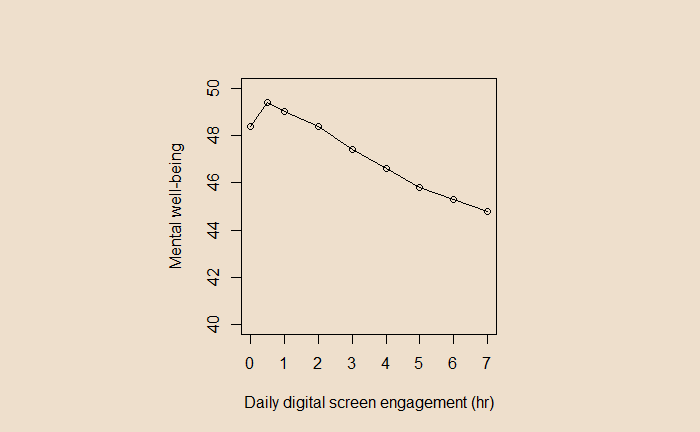
A casual look at the graph shows a steady decline in mental well-being as the screen time increases from 2 hours onwards. Until you notice the scale of the Y-axis!

In a 14-item survey with a 1-5 range in scale, the overall score must range from 14 (min) to 70 (max). Instead, In the present plot, the scale was from 40 to 50, thus visually exaggerating the impact. Had it been plotted following the (unwritten) rules of visualisation, it would have looked like this:

To conclude

Screen time impacts the mental well-being of adolescents. It increases a bit, followed by a decline. The magnitude of the decrease (from 0 screen time to 7 hr) is about 3 points on a 14-70 point scale.

References

Andrew K. Przybylski and Netta Weinstein, A Large-Scale Test of the Goldilocks Hypothesis: Quantifying the Relations between Digital-Screen Use and the Mental Well-Being of Adolescents, Psychological Science, 2017, Vol. 28(2) 204–215.
Joshua Marmara, Daniel Zarate, Jeremy Vassallo, Rhiannon Patten, and Vasileios Stavropoulos, Warwick Edinburgh Mental Well-Being Scale (WEMWBS): measurement invariance across genders and item response theory examination, BMC Psychol. 2022; 10: 31.

Screen Time and Happiness Read More »

Flight Accidents

YearAccidents
197624
197725
197831
197931
198022
198121
198226
198320
198416
198522

We assume that flight accidents are random and independent. This implies that the likelihood function (the nature of the phenomenon) is likely to follow a Poisson distribution. Let Y be the number of events occurring within the time interval.

Y|\theta = Pois(\theta)

Theta is the (unknown) parameter of interest, and y is the data (total of 10 observations). We will use Bayes’ theorem to estimate the posterior distribution p(theta|data) from a prior, p(theta). As we established long ago, we select gamma distribution for the prior (conjugate pair of Poisson).

Flight Accidents Read More »

This Sentence is False!

‘This sentence is false’ is an example of what is known as the Liar Paradox.

This sentence is false.

Look at the first option for the answer—true. To do that, we check what the sentence says about itself. It says about itself that it is false. If it is true, then it is false, which is a contradiction, and therefore, the answer ‘true’ is not acceptable.

The second option is false. Since the sentence claims about itself as false, then it’s false that it’s false, which again is a contradiction.

This Sentence is False! Read More »

The Log-Rank Test for Survival

Here are Kaplan – Meier plots for males and females taken from the results of a cancer study. The data comes from the ‘BrainCancer’ dataset from the R library ISLR2. It contains the survival times for patients with primary brain tumours undergoing treatment.

At first glance, it appears that females were doing better, up to about 50 months, until the two lines merged. The question is: is the difference (between the two survival plots) statistically significant?

You may think of using two-sample t-tests comparing the means of survival times. But the presence of censoring makes life difficult. So, we use the log-rank test.

The idea here is to test the null hypothesis, H0, that the expected value of the random variable X, E(X) = 0, and to build a test statistic of the following form,

W = \frac{X - E(X)}{\sqrt{Var(X)}}

X is the sum of the number of people who died at each time.

X = \sum\limits_{k = 1}^{K} q_{1k}

R does the job for you; use the library, survival.

library(ISLR2)
attach(BrainCancer)
as_tibble(BrainCancer)
library(survival)
survdiff(Surv(time, status) ~ sex)
Call:
survdiff(formula = Surv(time, status) ~ sex)

            N Observed Expected (O-E)^2/E (O-E)^2/V
sex=Female 45       15     18.5     0.676      1.44
sex=Male   43       20     16.5     0.761      1.44

 Chisq= 1.4  on 1 degrees of freedom, p= 0.2 

p = 0.2; we cannot reject the null hypothesis of no difference in survival curves between females and males.

Reference

An introduction to Statistical Learning: James, Witten, Hastie, Tibshirani, Taylor

The Log-Rank Test for Survival Read More »

Kaplan-Meier Estimate

The outcome variable in survival analysis is the time until an event occurs. Since studies are often time-bounded, some patients may survive the event at the end of the study, and others may stop responding to the survey midway through. In either case, those patients’ survival times are censored. As censored patients also provide valuable data, the analyst gets into a dilemma of whether to discard those candidates.

Let’s examine five patients in a study. The filled circles represent the completion of the event (e.g., death), and the open circles represent the censoring (either dropping out or surviving the study’s end date).

The survival function, S(t), is the probability that the true survival time (T) exceeds some fixed number t.
S(t) = P(T > t)
S(t) decreases with time (t) as the probability decreases as time passes.

In the above example, how do you conclude the probability of surviving 300 days, S(300)? Will it be 1/3 = 0.33 (only the one survived out of three events, ignoring the censored) or 3/5 = 0.6 (assuming the censored candidates also survived)? What difference does it make to the conclusion that one of them dropped out early when she was too sick?

Kaplan and Meier came up with a smart solution to this. Note that they worked on this problem separately. Their survival curve is made the following way.
1) The first event happened at time 100. The probability of survival at t = 100 is 4/5, noting that four of the five patients were known to have survived that stage.

2) We now proceed to the next event, patient 3. Note that we skipped the censored time of patient 2.

Now, two out of three survived. The overall survival probability at t = 200 is (4/5) x (2/3).

3) Move to the last event (patient 5); the survival function is zero ((4/5) x (2/3) x 0). This leads to the Kaplan -Meier plot:

Kaplan-Meier Estimate Read More »

Survival analysis – Sensoring

We have seen survival plots before. Survival plots represent ‘time to event’ in survival analysis. For example, in the case of cancer diagnostics, survival analysis measures the time it takes from exposure to the event, which is most likely death.

These analyses are done following a group of candidates (or patients) between two time periods, i.e., the start and end of the study. Candidates are enrolled at different times during the period, and the ‘time to event’ is noted down. Censoring is a term in survival analysis that denotes when the researcher does not know the exact time-to-event for an included observation.

Right censoring
The term is used when you know the person is still surviving at the end of the study period. Let x be the time since enrollment, and then all we know is the time-to-event ti > x. Imagine a study that started in 2010 and ended in 2020, and a person who was enrolled in 2018 was still alive at the study’s culmination. So we know that xi > 2 years. The same category applies to patients who missed out on follow-ups.

Left censoring
This happens in observational studies, where the risk happens before entering the studies. Because of this, the researcher cannot observe the time when the event occurred. Obviously, this can’t happen if the event is death.

Interval censoring
It occurs when the time until an event of interest is not known precisely and, instead, only is known to fall between two time stamps.

Survival analysis – Sensoring Read More »

Drug Development and the Valley of Death

One of the biggest beneficiaries of scientific methodology is evidence-based modern medicine. Each step in the ‘bench to bedside‘ process is a testimony of the scientific rigour in medicine research. While the low probability of success (PoS) at each stage is a challenge in the race to fight against diseases, it increases the confidence level in the validity of the final product.

The drug development process is divided into two parts: basic research and clinical research. Translational research is the bridge that connects the two parts. The ‘T Spectrum’ consists of 5 stages,

T0 includes preclinical and animal studies.
T1 is the phase 1 clinical trial for safety and proof of concept
T2 is the phase 2/3 clinical trial for efficacy and safety
T3 includes the phase 4 clinical trial towards clinical outcome and
T4 leads to approval for usage by communities.

Probability of success

According to a publication by Seyhan, who quotes NIH, 80 to 90% of research projects fail before the clinical stage. The following are typical rates of success in clinical drug development stages:
Phase 1 to Phase 2: 52%
Phase 2 to Phase 3: 28.9%
Phase 3 to Phase 4: 57.8%
Phase 4 to approval: 90.6%
The data used to arrive at the above statistics was collected from 12,728 clinical and regulatory phase transitions of 9,704 development programs across 1,779 companies in the Biomedtracker database between 2011 and 2020.

The overall chance of success from lab to shop thus becomes:
0.1×0.52×0.289×0.578×0.906 = 0.008 or < 1%!

References

Seyhan, A. A.; Translational Medicine Communications, 2019, 4-18
Mohsa, R.C.; Greig, N. H.; Alzheimer’s & Dementia: Translational Research & Clinical Interventions 3, 2017, 651-657
Cummings, J.L.; Morstorf, T.; Zhong, K.; Alzheimer’s Research & Therapy, 2014, 6-37
Paul, S.M; Mytelka, D.S.; Dunwiddie, C. T.; Persinger, C. C.; Munos, B.H.; Lindborg, S.R.; Schacht, A. L, Nature Reviews – Drug Discovery, 2010, VOlume 9.
What is Translational Research?: UAMS

Drug Development and the Valley of Death Read More »

Population Distributions vs Sampling Distribution

The purpose of sampling is to determine the behaviour of the population. For the definitions of terms, sample and population, see an earlier post. In a nutshell, population is everything, and a sample is a selected subset.

Population distribution

It is a frequency distribution of a feature in the entire population. Imagine a feature (height, weight, rainfall, etc.) of a population with a mean of 100 and a standard deviation of 25; the distribution may look like the following. It is estimated by measuring every individual in the population.

It means many individuals have the feature closer to 100 units and fewer have it at 90 (and 110). Still fewer have 80 (and 120), and very few exceptionals may even have 50 (and 150), etc. Finally, the shape of the curve may not be a perfect bell curve like the above.

Sampling distribution

Here, we take a random sample of size n = 25. Measure the feature of those 25 samples and calculate the mean. It is unlikely to be exactly 100, but something higher or lower. Now, repeat the process for another 25 random samples and compute the mean. Make several such means and plot the histogram. This is the sampling distribution. If the number of means is large enough, the distribution will take a bell curve shape, thanks to the central limit theorem.

In the case of the sampling distribution, the mean is equal to the mean of the original population distribution from which the samples were taken. However, the sampling distribution has a smaller spread. This is because the averages have lower variations than the individual observations.

standard deviation of sampling distribution = standard deviation of population distribution/sqrt(n). The quantity is also called the standard error.

Population Distributions vs Sampling Distribution Read More »

The Central Limit and Hypothesis Testing

The validity of newly explored data from the perspective of the existing population is the foundation of the hypothesis test. The most prominent hypothesis test methods—the Z-test and t-test—use the central limit theorem. The theorem prescribes a normal distribution for key sample statistics, e.g., average, with a spread defined by its standard error. In other words, knowing the population’s mean, standard deviation and the number of observations, one first builds the normal distribution. Here is one example.

The average rainfall in August for a region is 80 mm, with a standard deviation of 25 mm. What is the probability of observing rainfall in excess of 84 mm this August as an average of 100 samples from the region?

The central limit theorem dictates the distribution to be a normal distribution with mean = 80 and standard deviation = 25/sqrt(100) = 2.5.

Mark the point corresponds to 84; the required probability is the area under the curve above X = 84 (the shaded region below).

The function, ‘pnormGC’, from the package ‘tigerstats’ can do the job for you in R.

library(tigerstats)
pnormGC(84, region="above", mean=80, sd=2.5,graph=TRUE)

The traditional way is to calculate the Z statistics and determine the probability from the lookup table.

P(Z > [84-80]/2.5) = P(Z > 1.6) 
1 - 0.9452 = 0.0548

Well, you can also use the R command instead of searching in the lookup table.

1 - pnorm(1.6)

The Central Limit and Hypothesis Testing Read More »