Decision Making

Pilot Hit

February 29, 2024

Data from a television production company suggests that 10% of their shows are blockbuster hits, 15% are moderate success, 50% do break even, and 25% lose money. Production managers select new shows based on how they fare in pilot episodes. The company has seen 95% of the blockbusters, 70% of moderate, 60% of breakeven and 20% of losers receive positive feedback.

Given the background,
1) How likely is a new pilot to get positive feedback?
2) What is the probability that a new series will be a blockbuster if the pilot gets positive feedback?

The first step is to list down all the marginal probabilities as given in the background.

	Pilot	Outcome	Total
	Positive	Negative
Huge Success			0.10
Moderate			0.15
Break Even			0.50
Loser			0.25
Total			1.0

The next step is to estimate the joint probabilities of pilot success in each category.
95% of blockbusters get positive feedback = 0.95 x 0.1 = 0.095.
Let’s fill the respective cells with joint probabilities.

	Pilot	Outcome	Total
	Positive	Negative
Huge Success	0.095	0.005	0.10
Moderate	0.105	0.045	0.15
Break Even	0.30	0.20	0.50
Loser	0.05	0.20	0.25
Total	0.55	0.45	1.0

The rest is straightforward.
The answer to the first question: the chance of positive feedback = sum of all probabilities under positive = 0.55 or 55%.
The second quesiton is P(success|positive) = 0.095/0.55 = 0.17 = 17%

	Pilot	Outcome
	P(Positive)	P(success\|Positive)
Huge Success	0.095	0.17
Moderate	0.105	0.19
Break Even	0.30	0.55
Loser	0.05	0.09
Total	0.55	1.0

Reference

Basic probability: zedstatistics

Pilot Hit Read More »

Moving Average – Continued

February 28, 2024

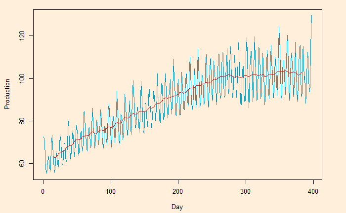
Here, we plot the daily electricity production data that was used in the last post.

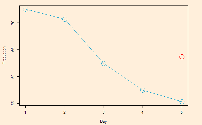
Following is the R code, which uses the filter function for building the 2-sided moving average. The subsequent plot represents the method on the first five points (the red circle represents the centred average of the first five points).

E_data$ma5 <- stats::filter(E_data$IPG2211A2N, filter = rep(1/5, 5), sides = 2)

For the one-sided:

E_data$ma5 <- stats::filter(E_data$IPG2211A2N, filter = rep(1/5, 5), sides = 1)

The 5-day moving average is below.

You can get a super-smooth data trend using the monthly (30-day) moving average.

Moving Average – Continued Read More »

Moving Average

February 27, 2024

Moving averages and means to smoothen noisy (time series) data, unearthing the underlying trends. The process is also known as filtering the data.

Moving averages (MA) are a series of averages estimated on a pre-defined number of consecutive data. For example, MA₅ contains the set of all the averages of 5 successive members of the original series. The following relationship represents how a centred or two-sided moving average is estimated.

MA₅ = (X_t-2 + X_t-1 + X_t + X_t+1 + X_t+2)/5

‘t’ represents the time at which the moving average is estimated. t-1 is the observation just before t, and t+1 means one observation immediately after t. To illustrate the concept, we develop the following table representing consecutive 10 points (electric signals) in a dataset.

Date	Signal
1	72.5052
2	70.6720
3	62.4502
4	57.4714
5	55.3151
6	58.0904
7	62.6202
8	63.2485
9	60.5846
10	56.3154

The centred MA starts from point 3 (the midpoint of 1, 2, 3, 4, 5). The value at 3 is the mean of the first five points (72.5052 + 70.6720 + 62.4502 + 57.4714 + 55.3151) /5 = 63.68278.

Date	Signal	Average
1	72.5052
2	70.6720
3	62.4502	63.68278
4	57.4714
5	55.3151
6	58.0904
7	62.6202
8	63.2485
9	60.5846
10	56.3154

This process is continued – MA on point 4 is the mean of points 2, 3, 4, 5 and 6, etc.

Date	Signal	MA
1	72.5052
2	70.6720
3	62.4502	63.68278 [1-5]
4	57.4714	60.79982 [2-6]
5	55.3151	59.18946 [3-7]
6	58.0904	59.34912 [4-8]
7	62.6202	59.97176 [5-9]
8	63.2485	60.17182 [6-10]
9	60.5846
10	56.3154

The one-sided moving average is different. It estimates MA at the end of the interval.
MA₅ = (X_t-4 + X_t-3 + X_t-2 + X_t-1 + X_t)/5

Date	Signal	MA
1	72.5052
2	70.6720
3	62.4502
4	57.4714
5	55.3151	63.68278 [1-5]
6	58.0904	60.79982 [2-6]
7	62.6202	59.18946 [3-7]
8	63.2485	59.34912 [4-8]
9	60.5846	59.97176 [5-9]
10	56.3154	60.17182 [6-10]

We will look at the impact of moving averages in the next post.

Moving Average Read More »

Value of a Portfolio

January 25, 2024

What are the expected return and standard deviation of an equal-weight portfolio of two assets, A and B, with the following characteristics?

Expected return of A = 10%
Expected return of B = 5%
Standard deviation of A = 20%
Standard deviation of B = 15%
The correlation between A and B is 0.5

The expected return of the portfolio,
E[r_p] = E[0.5 r_A + 0.5 r_B]
E[r_p] = 0.5 E[r_A] + 0.5 E[r_B]
E[r_p] = 0.5 x 0.1 + 0.5 x 0.05 = 0.075 = 7.5%

The standard deviation of the return
To calculate the standard deviation, std, we first calculate the variance, std².
var[r_p] = var[0.5 r_A + 0.5 r_B]
var[r_p] = 0.5² x var[r_A] + 0.5² var[r_B] + 2 x 0.5 x 0.5 cov[A,B]
cov[A,B] = corr(A,B) x std_A x std_B
var[r_A] = std_A²
var[r_B] = std_B²
var[r_p] = 0.5² x std_A² + 0.5² x std_B² + 2 x 0.5 x 0.5 corr(A,B) x std_A x std_B
var[r_p] = 0.5²x 0.2² + 0.5² x 0.15² + 2 x 0.5 x 0.5 x 0.5 x 0.2 x 0.15
var[r_p] = 0.023125
std_rp = sqrt(var[rp]) = sqrt(0.023125) = 0.152 = 15.2%

The portfolio’s expected return is midway between the lower and the higher; the risk (the standard deviation) is closer to the lower.

Value of a Portfolio Read More »

Value of a Lottery

January 24, 2024

A lottery has the following three prizes and sells 2 million tickets
1) one bumper prize of 1 million dollars.
2) 100 first prizes of 10,000 dollars each.
3) 10,000 consolation prizes of 1 dollar each.

If one ticket costs 2 dollars, should you buy the ticket?

The answer to this question depends on two aspects.
A) The difference between the expected value and cost of a single ticket.
B) The risk appetite of the buyer.

Expected value of a ticket

EV = P(1,000,000) x 1,000,000 + P(10,000) x 10,000 + P(1) x 1
where P(1,000,000) is the probability of winning a million dollar = 1 / 2,000,000

EV = [1/2,000,000] x 1,000,000 + [100/2,000,000] x 10,000 + [10,000/2,000,000] x 1
= 1.005

The cost of a ticket ($2) is higher than the expected value of winning ($1). A risk-averse or a risk-neutral person would avoid it.

Value of a Lottery Read More »

Conditional Probabilities

January 23, 2024

Based on the following data, what is the probability of a person making no error in her tax returns without support from a tax advisor?

50% of individuals get help from a tax advisor to file their returns. The probability of an individual making an error in the tax return is 25%. The chance of the person making an error, given a tax advisor is helping, is 10%.

Let P(M|A) be the probability of not making the error, given an advisor is not helping.
Based on the Conjunction Rule,
P(M & A) = P(A) x P(M|A)
P(M|A) = P(M & A) / P(A)

P(A) = probability of no advisor
P(M & A) = joint probability of no error AND no advisor.

Conditional Probabilities Read More »

Decision Quality

January 22, 2024

Sound decisions are core to achieving good outcomes. Decision quality (DQ) is the quality of a decision at the point it is made, regardless of its outcome. A decision framework should meet six requirements to reach DQ.

Appropriate frame: is about solving the right problem using the right people. The decision must have clarity of purpose, scope, boundaries and a conscious perspective.

Create doable alternatives: Give good choices within the frame. It will involve creativity, doability, breadth and completeness.

Relevant, reliable information: It may come from data and judgment. The issue with decision-making is that it is forward-looking, and all we have is data from the past. That means the data must be reliable and should describe the underlying uncertainties and biases.

Clear values and tradeoffs: Focus on value creation and transparency of value matrix and tradeoffs.

Sound reasoning: Use the information for each alternative and get the one with the greatest value.

Commitment to action: During the decision process, it’s important to get the right people and resolve any conflicts. Quality is defined by the support across stakeholders and a team that is ready to take action.

Reference

An Introduction to Decision Quality: Strategic Decisions Group

Decision Quality Read More »

Rationality in Game Theory

January 21, 2024

The word rationality has a different meaning in game theory than everyday usage. In common knowledge, rationality means the quality of a person seeking logic and reason for taking an action.

In game theory, the meaning is more specific and must fulfil a few conditions.

1) People are purposive: people engage in actions for an outcome. More specifically, the players involved in the game seek to achieve the most desired outcome.

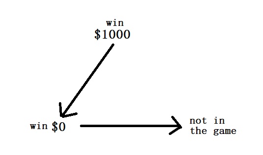
2) Completeness of preference: the player’s preference order must be complete. For any two outcomes, X and Y, the player can choose X over Y, Y over X or indifferent between the two. But ‘I don’t know’ is not allowed! The following scheme represents the preference for X over Y:

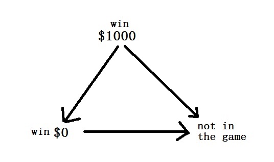
3) Transitivity of preference: For three outcomes, X, Y and Z, if X is preferred to Y and Y to Z, then X must be preferred to Z. So if a player prefers winning $1000 over winning $0. Winning $0 over not being able to participate, she must prefer winning $1000 over not being able to participate.

Implies

The preference ordering in this case is:
Win $1000
Win $0
Not in the game

4) Preference must be fixed

References

Rationality: David Hayes
Rationality: William Spaniel

Rationality in Game Theory Read More »

Traveller’s Dilemma

January 20, 2024

Traveller’s Dilemma, formulated by Kaushik Basu in 1994, is a game theory paradox that shows the gulf between the rational choice (the Nash equilibrium) and real-life behaviour. The description of the game is as follows:

Two travellers, A and B, find their bags damaged by the airline when returning from a vacation. The bags and the artefacts inside are identical. The airline manager mentions that the policy allows a minimum of $2 and a maximum of $100 reimbursement. Since she does not know the value of the objects, the manager separates the travellers and asks them to write down the value. But, on a few conditions.

1) They can write a number between 2 and 100
2) They receive the same amount if they write the identical numbers.
3) If they are different, both will get the lower amount. In addition, the person with the lower quote gets $2 as a bonus, and the person with a higher one loses $2. For example, if A quotes 45 and B 80, A gets 47 (45 +2), and B gets 43 (45 -2).

Nash Equilibrium

The rational process goes like this. A first thinks of writing $100. A then changes her mind, thinking B could also write $100. In that case, both will receive $100. On the other hand, if A writes $99 (and B $100), A will get $101, including the bonus amount for being a lower quote. But A knows B can also think in similar logic, thereby changing her quote to 98, and so on. The Nash equilibrium is where both players write down $2!

The theory has been tested in web-based experiments by Ariel Rubinstein. The players had the task of writing a number between 180 and 300. The results, however, did not match the rational expectation. Most participants (55%) chose to write the maximum number. 17% wrote numbers between 295 and 299, 14% between 181 and 294, and only 13% wrote the Nash equilibrium of 180.

Reference

The Traveler’s Dilemma: Scientific American

Traveller’s Dilemma Read More »

Chain Store Paradox – The Paradox

January 19, 2024

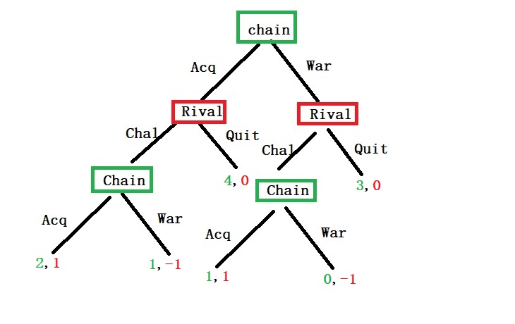
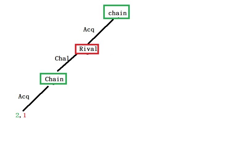
We have seen in the earlier post that the chain store has an optimal solution when it goes for acquiesce, followed by acquiesce, and the second rival enters the market.

The chain store, however, can dump the backward induction results of optimal payoff and show its strength by going to war in the first town itself. The purpose is to signal the rival that it would do the same if it entered town 2.

If that worked and deterred the rival from entering town 2, the chain store would receive a payoff = 3, which is more than what the cooperation route brings, as we saw earlier.

This is the paradox: the induction strategy should be the equilibrium choice per game theory, yet the chain store would choose a deterrence strategy as the optimal.

Chain Store Paradox – The Paradox Read More »