Annie says Becky is lying Becky says Carol is lying Carol says both Annie and Becky are lying
Who is lying, and who is telling the truth?
If Carol is telling the truth, then Annie (and Becky) is lying. In that case, Becky is not lying (opposite of what Annie, the ‘liar’ said). This is a contradiction. Therefore, Carol is lying.
Since Carol is lying, the person who identified that correctly, Becky, must be telling the truth
If Becky is telling the truth, the first statement is incorrect. Therefore, the person who made the first statement, Annie, is also lying.
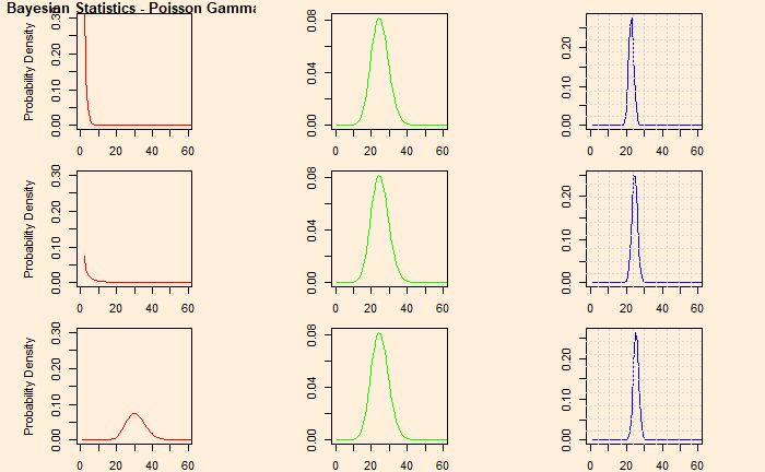
We assume that flight accidents are random and independent. This implies that the likelihood function (the nature of the phenomenon) is likely to follow a Poisson distribution. Let Y be the number of events occurring within the time interval.
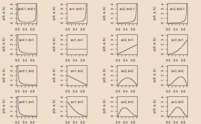
Theta is the (unknown) parameter of interest, and y is the data (total of 10 observations). We will use Bayes’ theorem to estimate the posterior distribution p(theta|data) from a prior, p(theta). As we established long ago, we select gamma distribution for the prior (conjugate pair of Poisson).
‘This sentence is false’ is an example of what is known as the Liar Paradox.
This sentence is false.
Look at the first option for the answer—true. To do that, we check what the sentence says about itself. It says about itself that it is false. If it is true, then it is false, which is a contradiction, and therefore, the answer ‘true’ is not acceptable.
The second option is false. Since the sentence claims about itself as false, then it’s false that it’s false, which again is a contradiction.
It has been found that the scores obtained by students follow a normal distribution with a mean of 75 and a standard deviation of 10. The top 10% end up in the university. What is the minimum mark for a student if she gets admission to the university?
The first step is to convert the percentage to the Z-score. It can be done in one of two ways.
qnorm(0.1, lower.tail = FALSE)
qnorm(0.9, lower.tail = TRUE)
1.28
Note that if you do not specify, the default for qnorm will be lower.tail = TRUE.
Z = (X – mean)/standard deviation X = Z x standard deviation + mean X = 1.28 x 10 + 75 = 87.8
We have seen family-wise error rate (FWER) as the probability of making at least one Type 1 error when conducting m hypothesis tests.
FWER = P(falsely reject at least one null hypothesis) = 1 – P(do not reject any null hypothesis) = 1 – P(∩j=1n {do not falsely reject H0,j})
If each of these tests is independent, the required probability equals (1 – α)n, and FWER = 1 – (1 – α)n
For example, if the significance level is 0.05 (α) for five tests, FWER = 1 – (1 – 0.05)5 And, if you make n = 100 independent tests, FWER = 1 – (1 – 0.05)100 = 0.994; guaranteed to make at least one Type I error.
One of the classical methods of managing the FWER is the Bonferroni correction. As per this, the corrected alpha is the original alpha divided by the number of tests, n. Bonferroni corrected α = original α / n
For five tests, FWER = 1 – (1 – 0.05/5)5 = 0.049; and for 100 tests FWER = 1 – (1 – 0.05/100)100 = 0.049
Imagine a fair coin is tossed 10 times to test the hypothesis, H0: the coin is unbiased. The coin likely lands on heads (or tails) in about 5 (or 4, 3, 2) of those. If it landed 4 times on heads and 6 in tails, we can do a simple chi-squared test to verify. chi-squared = (4 – 5)2 /5 + (4 – 5)2 /5 = 0.4. 0.4 is too low; we can’t reject null
But what happens if all the tosses land on tails? chi-squared = (0 – 5)2 /5 + (10 – 5)2 /5 = 10. We reject at 99% confidence level. We know the probability of this happening is (1/2)10 = 1/1024.
chisq.test(c(0,10),p=c(0.5,0.5))
	Chi-squared test for given probabilities

data:  c(0, 10)
X-squared = 10, df = 1, p-value = 0.001565
What about 1024 players, each having a (fair) coin toss 10 times each?
1 - dbinom(0, 1024, 1/1024)
0.63
In other words, there is a possibility that one person will reject the null hypothesis and conclude that the coin is based! An incorrect rejection of a null hypothesis or a false positive result. In other words, if we test a lot (a family) of hypotheses, there is a high probability of getting one very small p-value by chance.
One of the biggest beneficiaries of scientific methodology is evidence-based modern medicine. Each step in the ‘bench to bedside‘ process is a testimony of the scientific rigour in medicine research. While the low probability of success (PoS) at each stage is a challenge in the race to fight against diseases, it increases the confidence level in the validity of the final product.
The drug development process is divided into two parts: basic research and clinical research. Translational research is the bridge that connects the two parts. The ‘T Spectrum’ consists of 5 stages,
T0 includes preclinical and animal studies. T1 is the phase 1 clinical trial for safety and proof of concept T2 is the phase 2/3 clinical trial for efficacy and safety T3 includes the phase 4 clinical trial towards clinical outcome and T4 leads to approval for usage by communities.
Probability of success
According to a publication by Seyhan, who quotes NIH, 80 to 90% of research projects fail before the clinical stage. The following are typical rates of success in clinical drug development stages: Phase 1 to Phase 2: 52% Phase 2 to Phase 3: 28.9% Phase 3 to Phase 4: 57.8% Phase 4 to approval: 90.6% The data used to arrive at the above statistics was collected from 12,728 clinical and regulatory phase transitions of 9,704 development programs across 1,779 companies in the Biomedtracker database between 2011 and 2020.
The overall chance of success from lab to shop thus becomes: 0.1×0.52×0.289×0.578×0.906 = 0.008 or < 1%!
References
Seyhan, A. A.; Translational Medicine Communications, 2019, 4-18 Mohsa, R.C.; Greig, N. H.; Alzheimer’s & Dementia: Translational Research & Clinical Interventions 3, 2017, 651-657 Cummings, J.L.; Morstorf, T.; Zhong, K.; Alzheimer’s Research & Therapy, 2014, 6-37 Paul, S.M; Mytelka, D.S.; Dunwiddie, C. T.; Persinger, C. C.; Munos, B.H.; Lindborg, S.R.; Schacht, A. L, Nature Reviews – Drug Discovery, 2010, VOlume 9. What is Translational Research?: UAMS
We have seen the placebo effect. It occurs when someone’s physical or mental condition improves after taking a placebo or ‘fake’ treatment. Placebos are crucial in clinical trials, often serving as effective means to screen out the noise, thereby contributing as the control group to compare the treatment results. Is providing a placebo good enough to remove the biases of a trial?
If the placebo group knows they received the ‘fake pill’, it will nullify its influence. So, the first step in helping the experiment is to hide the information that it is real or placebo from the participants who receive the treatment. This is a single-blind test.
More is needed to prevent what is known as the experimenter bias, also known as the observer expectancy effect. In the next level of refinement, the information is also hidden from the experimenter. This becomes a double-blind experiment. The National Cancer Institute defines it as: “A type of clinical trial in which neither the participants nor the researcher knows which treatment or intervention participants are receiving until the clinical trial is over.”
That means only a third party, who will help with the data analysis, will know the trial details, such as the allocation of groups or the hypothesis. Double-blind studies form the gold standard in evidence-based medical science.
The purpose of sampling is to determine the behaviour of the population. For the definitions of terms, sample and population, see an earlier post. In a nutshell, population is everything, and a sample is a selected subset.
Population distribution
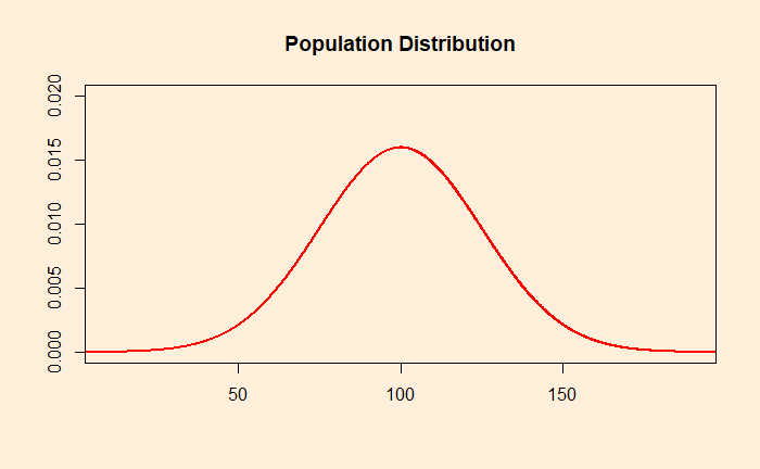
It is a frequency distribution of a feature in the entire population. Imagine a feature (height, weight, rainfall, etc.) of a population with a mean of 100 and a standard deviation of 25; the distribution may look like the following. It is estimated by measuring every individual in the population.
It means many individuals have the feature closer to 100 units and fewer have it at 90 (and 110). Still fewer have 80 (and 120), and very few exceptionals may even have 50 (and 150), etc. Finally, the shape of the curve may not be a perfect bell curve like the above.
Sampling distribution
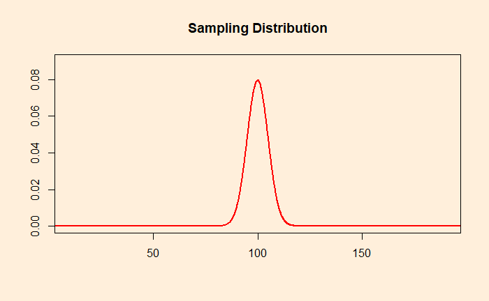
Here, we take a random sample of size n = 25. Measure the feature of those 25 samples and calculate the mean. It is unlikely to be exactly 100, but something higher or lower. Now, repeat the process for another 25 random samples and compute the mean. Make several such means and plot the histogram. This is the sampling distribution. If the number of means is large enough, the distribution will take a bell curve shape, thanks to the central limit theorem.
In the case of the sampling distribution, the mean is equal to the mean of the original population distribution from which the samples were taken. However, the sampling distribution has a smaller spread. This is because the averages have lower variations than the individual observations.
standard deviation of sampling distribution = standard deviation of population distribution/sqrt(n). The quantity is also called the standard error.