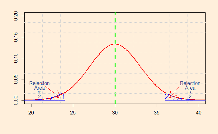
So how do you decide whether to choose one-tailed or two-tailed? It is not as straightforward as it may sound. Let’s look at the distributions that we have seen in the last post. So, first, the two-tailed test.
The shaded area represents the probability that a value will fall within the range. The smaller the value, you attain more confidence to reject the default – the null hypothesis. In this case, I have calculated the sum of the two regions to be 0.05. I guess you know what it means? It represents the alpha (significance level) of 5%.
Mean salary of 30k
So, if the null hypothesis (H0) was that the mean salary of engineers is exactly 30k, you can easily prove it is not the case if you find a sample mean of more than 35.9 or less than 24.1. Mathematically, it is:
So far, so good.
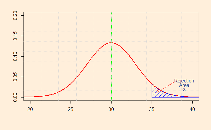
What will you do if you decide to prove only the higher side of the claim? i.e., you want to establish that the salary is more than 30k. That will mean the following shaded area of the distribution.
You can now see the problem: you can claim you have achieved the same 5% alpha at a sample mean of 35k.
In case you are wondering from where I got these 34.9, 24.1 and 35, try typing the following R codes.
pnorm(34.95, 30, 3, lower.tail = FALSE) # gives an answer 0.049 for one-tailed.

1 - pnorm(35.9, 30, 3) + pnorm(24.1, 30, 3) # gives 0.049 for two-tailed.
#the above code is equivalent to
pnorm(35.9, 30, 3, lower.tail = FALSE) + pnorm(24.1, 30, 3, lower.tail = TRUE)
pnorm represents the cumulative density function of a normal distribution with a mean = 30 and the standard deviation = 3.
We have seen the significance value alpha as the threshold probability of rejecting the null hypothesis. Let us illustrate it graphically. Consider this hypothesis: The average weighting time of the ticket counter is more than 30 minutes. The null and alternate hypotheses are:
H0: average less than or equals 30
HA: average more than 30
To establish your theory, you need to prove that the mean is greater than 30 (HA) beyond doubt. In the following illustration, the right-hand side tail provides the region you need to show your measured waiting time. That gives the alpha probability for the H0 to be valid.
Consider this: the starting monthly salary of computer engineers is $30k. The alternate hypothesis needs to prove this is not the case, the number may be lower or higher (two extremes or tails).
We will continue with the basic terms of hypothesis testing. The first one is the significance level. Alpha, as popularly known, is set by the person in charge of the testing and signifies the strength of the evidence required to establish the tester’s proposition (alternative hypothesis). We are familiar with the alpha of 0.05 (5%). But how does one choose the right level?
The famous analogy is the court cases. For civil cases (deal with personal rights), scholars define 51% of the evidence to support a claim. On the other hand, criminal cases may require far more, say, more than 90% of the evidence, for a verdict against the suspect. It may go to 99% when the potential punishment of the guilty is severe. You may look back at an older post to see the significance of where the judges draw their lines.
In the same way, the analyst may decide on a stricter significance level or a lower probability of rejecting the null hypothesis if the stakes are high. Putting it differently, an alpha of 0.01 means a 1% probability that the test will produce a statistically significant result if the null hypothesis is correct.
Reference
Jim Frost, “Hypothesis Testing: An Intuitive Guide for Making Data Driven Decisions”
We have done it several times in the past. The objective of hypothesis testing is to assess, using sample data, two mutually exclusive theories about the properties of a population. Please see my earlier post for the definitions of sample and population. The two theories are the null hypothesis and the alternative hypothesis.
The null hypothesis (H0) typically represents the default state or the state of “no effect“. For example, you compare the means of two groups, such as people who took a particular drug and people who received the placebo. As a drug researcher, your objective is to find the effectiveness of the medicine. And that lays the foundation for your alternative hypothesis (HA or H1) – that the drug has a non-zero effect. The default state (H0) assumes the drug has no impact. To be specific, H0 assumes the difference between two means equals zero.
H1 states that the population parameter value does not equal the H0 value. Notice the words, population and parameter. The ambition of the test is to create statements on the who space and not just on the sample itself. And if the sample contains sufficient evidence, we will see what is sufficient, you will reject the null hypothesis in favour of the alternative.
If having a gun increases the risk of gun-related violent death in the home, why do people choose to own guns?
Pierre, J. M., “The psychology of guns: risk, fear, and motivated reasoning”, Palgrave Communications, 5, 2019
My thoughts go with the children, teachers at the Robb Elementary School in Texas, and their family members.
I will start with my viewpoint on this debate of whether guns kill people vs people kill people – people attack, and they use readily available weapons to cause harm to “the other“. The more lethal the tool used, the deadlier the injury, with death as the endpoint. In other words, if stones are accessible, the outraged may throw and hurt the other, and if guns are accessible, they may kill a few; in a more barbarian society, replace guns with bombs! Only the scale changes. It is as simple as that.
There are statistics, and so are beliefs
In one of the previous posts, we discovered that suicides dominated the gun-related deaths. Studies after studies report the association that homicides are largely incidents committed by family members and acquaintances and not strangers.
Yet, the society, the US in this context, supports and takes great pride in possession of guns! The proponents of guns have several reasons (excuses) to support their position, starting with individual freedom (we have seen it in Covid-19 mask mandates!), to what is known, as per some studies, as the knowledge deficit model.
But one theory that became the most prominent among them points to the aspect of human decision making – i.e., irrationality, controlled by cognitive biases (cherry-picking, motivated reasoning, availability heuristics, status quo bias). As per Metzl, this behaviour stems from the notion of the cultural heritage of gun owners. And it does not come as a surprise that other social cancers (a.k.a. resistance to progress) – religiosity, racism, sexism, nationalism – too originate from similar backgrounds.
The Second Amendment
The story goes back to the second amendment of the US constitution that states, “A well regulated Militia, being necessary to the security of a free State, the right of the people to keep and bear Arms, shall not be infringed.”
First, you need to remember that this followed centuries-old practices of England (English Bill of Rights of 1689), which was embraced and ratified by the US constitution in 1791. And the reason to carry this baggage of the past? The answer is complicated.
Social scientists have been approaching this American love of guns through the lenses of gender, masculinity and race. On top of these, there are the thriving forces of fear of “bad guys, thugs and carjackers“, amply fostered by the ever-powerful National Rifle Association (NRA).
Uncertain future
A solution based on rational, data-based arguments is unlikely to reap any rewards against motivated reasoning. The issue is deep-rooted in American society as a national identity, symbol of resistance, and a collective history of race, gender and socioeconomic status. And as always, such diseases require long term care to heal.
Further Reading
Metzl, J., What guns mean: the symbolic lives of firearms, 2019, Palgrave Comm., 5:35 Pierre, J. M., The psychology of guns: risk, fear, and motivated reasoning, 2019, Palgrave Comm., 5:159
Let’s attempt to understand the payoffs and coach Spoelstra’s options for game 4 of the NBA eastern conference final (ECF). Before we get into the arguments, here is a brief primer on the subject that we are discussing today.
The 2022 NBA ECF
And the matchup is between the Miami Heat and the Boston Celtics, with the Heat leading 2-1 at the end of game 3. Game 4, just like game 3, is at Celtic’s court, TD Gardens. So, there is a homecourt advantage for the Boston team. Heat’s star player Jimmy Butler just got injured (knee inflammation) in game 3. Let’s assume the injury was not a serious one, and there is a possibility he could be back for the next game. After game 4, there is a maximum of 3 more games, two of them in Miami’s backyard. Whichever team reaches four wins first will win the conference and advance to the NBA finals.
Butler brings advantage, and so is home.
Let’s write down the key assumptions and payoffs. If Butler plays, his team gets a boost of about 0.2 probability points over not playing. i.e., at home, it is 0.6 vs 0.4, and away 0.4 vs 0.2. If he plays in game 4, there is a 0.5 chance of aggravating his injury, making him unavailable for game 5. If he doesn’t play game 4, there is a 0.8 chance he plays for game 5 healthy, thanks to two additional days of rest. If the Heat wins game 4, it will be a huge boost to win the conference, as they have two home and one away matches to realise just one more win. If they lose game 4, it is still fine as they tie at 2-2, with two more to win with two home matches at hand.
What should Spoelstra do?
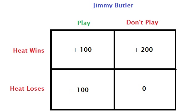
Well, he should weigh down factors and write payoff matrices and expected values. I will make one, not exactly a payoff matrix, but still capable of describing winning and losing with and without Butler.
These payoff values are arbitrary, but a win without Butler ranks the highest as he will be available as a fitter player for the rest of the games to close out. Butler playing and losing is risky as there is a higher chance of worsening the injury. And the other two results yield somewhere in between these two extremes.
Dominant strategy
If you compare the first column of the matrix with the second, i.e., comparing Butler playing with not playing, you will note that + 200 > + 100 and 0 > – 100. So, under these payoff values, Butler not playing is the dominant strategy.
Expected values
Let Vplay be the expected value for the Heat when Butler plays, and Vno-play when Butler does not play.
Vplay = 100 x 0.4 + (-100) x 0.6 = – 20
Vno-play= 200 x 0.2 + 0 x 0.8 = 40
Again, Butler not playing has the higher expected value.
Any doubts, coach?
The value of the above arguments is only worth the underlying assumptions, which, at this stage, are only arbitrary or speculative.
Tailpiece
(added on May 24, after the end of match 4). Butler played for the Heat, but the Celtics won by 20 points. Butler scored 6 points in the game (his previous scores were 41, 29 and 8). Whether his involvement in the match affected his fitness for future ties remains to be seen or will never be known.
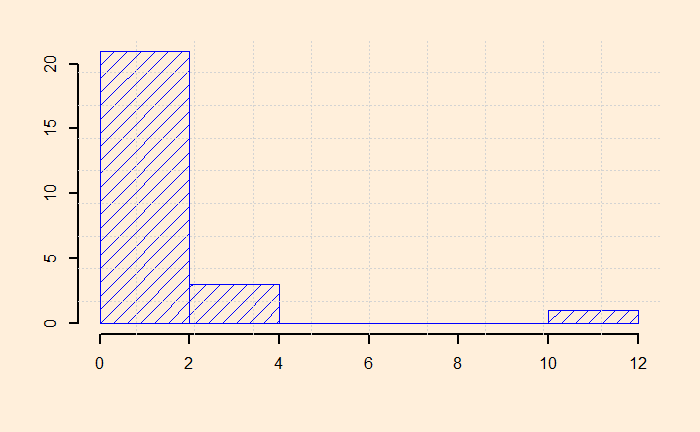
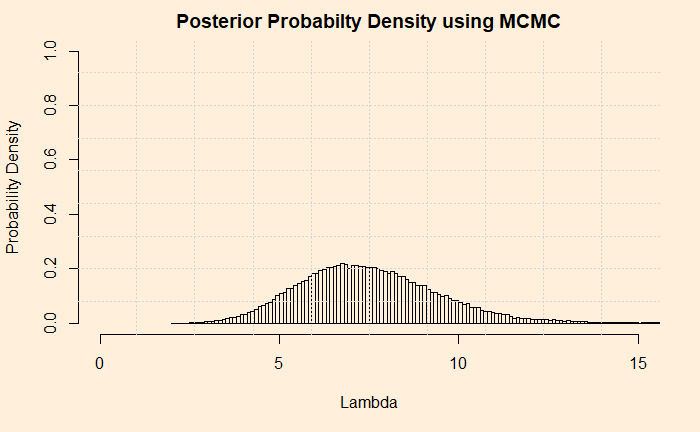
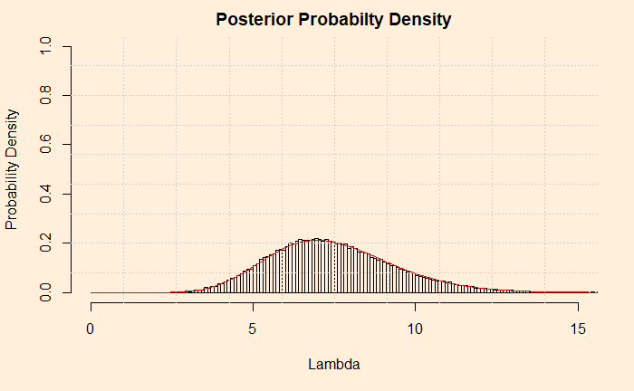
In the last post, we developed an MCMC algorithm for calculating the posterior probability distribution for the shark problem. We will do a few more things on it before closing out.
The first thing is to express the histogram in the form of Gamma distribution. We calculate the mean and variance of the data and apply the following formulae.
Now, check the post where we did the analytical solution for the hyperparameters of the posterior. Do they match?
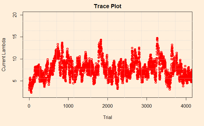
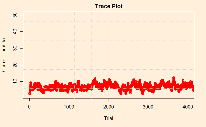
Trace Plot
Trace plot is next. It is a line diagram connecting all the current lambdas against the trial number. The following plot gives the first 4000 (of the 100,000) trials we have performed.
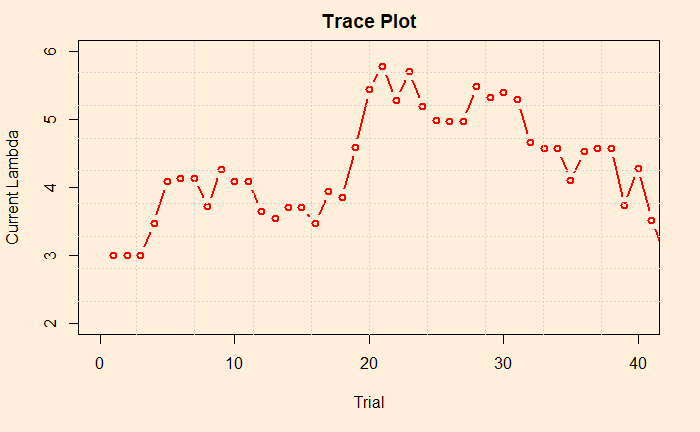
Now we pick the first 40 to zoom in on the values.
By looking at the plot, you may recognise the concept known as the acceptance rate. It is the percentage of instances where the current lambda got rejected in favour of the proposed. In the figure, there are approximately three in four times the points jumped (up or down) to a new value. There are recommendations to keep the acceptance rates between 25 – 50% as a good practice. You can tune the rate by varying the standard deviation of the normal distribution (step 3 of the MCMC scheme).
Impact of starting lambda
Finally, we look into the sensitivity of prior. We had arbitrarily chosen 3 in the previous exercise. Here is the trace plot once again.
What about changing it to 30? We could see that the distribution remained the same (after 100,000 iterations). Let’s check the trace plot. You will notice that it was higher, to begin with, but came down in a few trials.
Reference
Bayesian Statistics for Beginners: a step-by-step approach, Donovan and Mickey
So far, we have created an analytical solution to the Poisson-Gamma conjugate problem. Now, it is time for the next step: a numerical solution using the Markov Chain Monte Carlo (MCMC) method. The plan is to go stepwise and develop R codes side by side.
Markov Chain Monte Carlo
We write the Bayes’ theorem in the following form,
Step 0: The Objective
The objective of the exercise is to calculate the probability density of the posterior (updated hypothesis) given the (new) data at hand. As we did previously, we will need to use the hyperparameters alpha and beta.
data_new <- 10
alpha <- 5
beta <- 1
Step 1: Guess a Lambda
You start with one value for the posterior distribution (of lambda). It can be anything reasonable; I just took 3. It is an arbitrary selection. We can think of changing to something else later.
current_lambda <- 3
Step 2: Calculate the Likelihood, prior and posterior
Use the guess value of lambda and calculate the likelihood using Poisson PMF. In other words, get the chance of occurrence of a rare independent event 5 times in a year if the lambda was 3.
liklely_current <- dpois(data_new,current_lambda)
Calculate the prior probability density associated with the lambda (value of the posterior) for the given hyperparameters, alpha and beta. Sorry, I forgot: use Gamma PDF.
The next one is obvious, use the calculated values of prior and likelihood and calculate the probability density of the posterior using the new form of the Bayes’ equation.
post_current <- liklely_cur*prior_current
Step 3: Draw a Random Lambda
The second value of lambda is selected at random from a symmetrical distribution that is centred at the current value of lambda. We will use a normal distribution for that. We’ll call the new value, the proposed lambda. I used the absolute value because the new value can pick negative once in a while and lead the program to terminate.
Now you have two posterior values, post_current and post_proposed. We go to throw one out. How do we make that decision? Here comes the famous Metropolis algorithm to the rescue. It specifies to pick the smaller of the two between 1 and the ratio of the two posteriors. The resulting value is the probability of moving to the new lambda.
prob_move <- min(post_proposed/post_current, 1)
Step 6: New Lambda or the Old
The verdict (to move or not) is not out yet! Now, draw a random number from a uniform distribution and compare it. If your number is higher than the random number, move to the new lambda, and if not, stay with the old lambda.
You have done one iteration, and you have a lambda (switch to new or retain the old). Now, you go back to step 2 and repeat all steps. Thousands of times until you meet the set iteration number, for example, one hundred thousand!
n_iter <- 100000
for (x in 1:n_iter) {
}
Step 8: Collect All the Accepted Values
Ask the question: what is the probability density distribution of the posterior? It is the normalised frequency of lambda values. Note that I just omitted the condition, “given the data”, to keep it simple, but don’t forget, it is always the conditional probability. You may get the histogram from the frequency data using the attribute “freq = FALSE”. See below
We have created the background on the Shark attack problem to explain how Bayesian inference operates for updating knowledge of an event, in this case, a rare one. Let’s have a quick recap first. We chose Poisson distribution to describe the likelihood (the chances of that data on attacks, given a particular set of occurrences) because we knew these were rare and uncorrelated events. And the Gamma for describing the prior probability of occurrences as it can give a continuous set of instances ranging from zero to infinity.
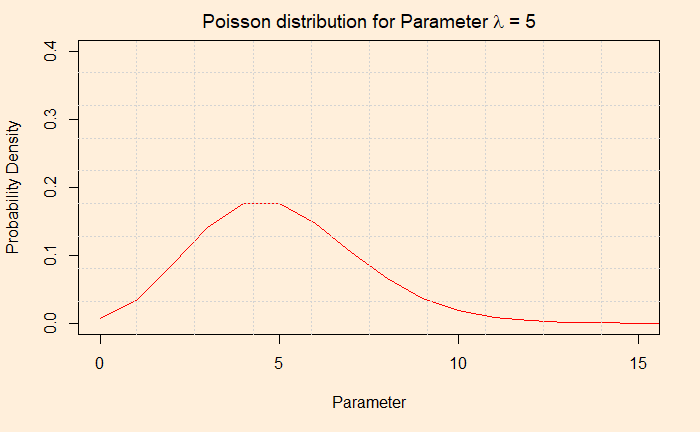
And if you like to know how those two functions work, see the following two plots.
The first plot gives the probability of one occurrence, two occurrences, 3, 4, 5, 6 …, when the mean occurrence is five. The value the X-axis take is discrete: you can not have the probability of 1.8 episodes of a shark attack!
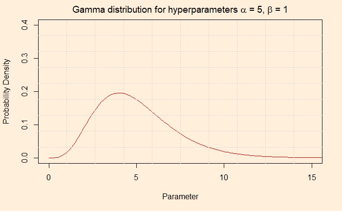
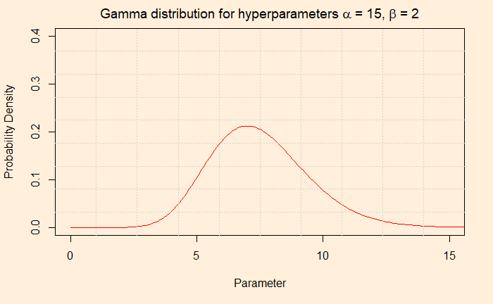
The second plot provides the probability of the parameter (occurrence or episode) through the gamma pdf using those two hyperparameters, alpha and beta.
Bayesian Inference
The form of Bayes’ theorem now becomes.
Then the magic happens, and the complicated looking equation solves into a Gamma distribution function. You will now realise the choice of Gamma as the prior was not an accident, but it was because of its conjugacy with the Poisson. But we have seen that before.
The Posterior
The posterior is a Gamma pdf with the following hyperparameters.
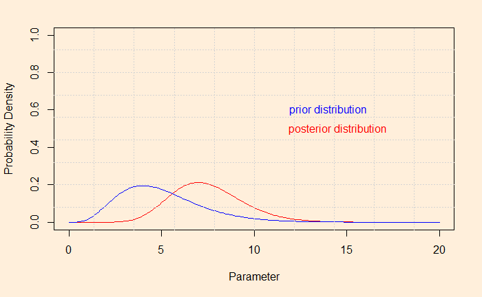
And, if you want to see the shift of the hypothesis from prior to posterior after the evidence,