Ellsberg and Allais paradoxes have one thing in common – both reflect our ambiguity aversion. Given the opportunity to choose between a ‘sure thing’ and an uncertain one, people tend to pick the former. Or it is the behaviour characteristics that dictate your decision-making when the probability of the outcome is known vs it is unknown; a feeling that tells you an uncertain outcome is a negative outcome.
In the case of the Ellsberg paradox, people are happy to bet on the red ball when they know the risk (33% chance) against the ambiguity surrounding the black and yellow. The same people had no issue dumping the mathematically identical option (red) when they knew there was a 60% chance of getting 100 if they went for one of the others.
In the case of the Allais, it was a fear imposed by a 1% chance of getting nothing. If you want to know that fear, let’s take the case of a vaccine that can give a 10% chance of 5-year protection, 89% chance of 1-year protection and a 1% chance of no protection, or worse, a 1 in a million probability of death! If that was placed side by side with another one that guarantees 1-year protection to all, without any known side effects, guess what I would go for.
You have two choices: A) A lottery that guarantees $ 1 M vs B) where you have a 10% chance of winning $ 5M, 89% chance for 1 M and 1% chance of nothing. Which one will you choose? If I write them in a different format:
A
$ 1M (1)
B
$ 5M (0.1); $ 1M (0.89); $ 0 (0.01)
Having chosen one of the above two, you have another one to choose from. C) A lottery with an 11% chance of $ 1 M and 89% chance of nothing vs D) a 10% chance of winning $ 5M, 90% chance of nothing.
C
$ 1M (0.11); $ 0M (0.89)
D
$ 5M (0.1); $ 0 (0.9)
Allais (1953) argued that most people preferred A and D. What is wrong with that?
Expected Value
If the person had followed the expected value theory, she could have chosen B and D:
A) $ 1M x 1 = $ 1M B) $ 5M x 0.1 + $ 1M x 0.89 + $ 0 x 0.01 = $ 1.39 M C) $ 1M x 0.11 + $ 0M x 0.89 = $ 0.11 M D) $ 5M x 0.1 + $ 0 x 0.9 = $ 0.5 M
Expected Utility
Since the person chose A over B, clearly, it was not the expected value but an expected utility that governed her. Mathematically,
U($ 1 M) > U($ 5 M) x 0.1 + U($ 1 M) x 0.89 + U($ 0M) x 0.01
Now, collect the U($ 1 M) on one side, add U($ 0M) x 0.89 on both sides, and simplify.
U($ 1 M) – U($ 1 M) x 0.89 > U($ 5 M) x 0.1 + U($ 0M) x 0.01 U($ 1 M) x 0.11 > U($ 5 M) x 0.1 + U($ 0M) x 0.01 U($ 1 M) x 0.11 + U($ 0M) x 0.89 > U($ 5 M) x 0.1 + U($ 0M) x 0.01 + U($ 0M) x 0.89 U($ 1 M) x 0.11 + U($ 0M) x 0.89 > U($ 5 M) x 0.1 + U($ 0M) x 0.9
Pay attention to the last equation. What are you seeing here? The term on the left side is the expected utility equation corresponding to option C, and the one on the right side is option D. In other words, if A > B, then C > D. But that was violated in the present case.
Imagine an urn containing 90 balls: 30 red balls and the rest (60) black and yellow balls; we don’t know how many are black or yellow. You can draw one ball at random. You can bet on a red or a black for $100. Which one do you prefer?
Red
Black
Yellow
A
$100
$0
$0
B
$0
$100
$0
Ellsberg found that people frequently preferred option A.
Now, a different set of choices: C) you can bet on red or yellow vs D) bet on black or yellow.
Red
Black
Yellow
C
$100
$0
$100
D
$0
$100
$100
Most people preferred D.
Why is it irrational?
If you compare options A and B, you can ignore the column yellow because they are the same. The same is the case for C vs D (ignore yellow as they offer equal amounts). In other words – if you had preferred A, logic would suggest you choose C and not D.
Red
Black
A
$100
$0
B
$0
$100
C
$100
$0
D
$0
$100
A = C; B = D
The second way is to look at it probabilistically. If you chose option A, you are implicitly telling that the probability of Red is more than the probability of Black. If that is the case, in the second exercise, the probability of Red or Yellow has to be greater than the probability of Black or Yellow. But you violated the law with your preference.
Decision under uncertainty
Clearly, the decision was not made based on probability or expected values. What is common for B and C is the perception of ambiguity. In the case of A, there is no 30% guarantee for a Red. In the case of D, there is a 60% guarantee to win $100.
The final episode of this series is a paired t-test. We have done it before, manually. Today we will do it using R.
The exercise we did earlier was on a weight-loss program. “Company X claims its weight-loss drug success by showing the following data. You’ll test whether there’s any statistical evidence for the claim (at a 5% significance level)“.
Before
After
120
114
94
95
86
80
111
116
99
93
78
83
78
74
96
91
132
136
108
109
94
90
88
91
101
100
93
90
121
120
115
110
102
103
94
93
82
81
84
80
The null hypothesis, H0: (weight before – after) = 0. The alternative hypothesis, HA: (weight before – after) > 0.
We insert the data in the following command and run the function, t.test.
Note that we went for a one-tailed (right side) test as we wanted to verify the increase (the option, alternative = “greater”), not just a change from the reference value.
Paired t-test

data:  A_B_data$Before and A_B_data$After
t = 1.6303, df = 19, p-value = 0.05975
alternative hypothesis: true difference in means is greater than 0
95 percent confidence interval:
 -0.08179912         Inf
sample estimates:
mean of the differences
                   1.35
There was a difference of 1.35, yet the p-value was higher than the critical value we chose (0.05). The test shows no evidence to prove its effectiveness. Therefore, the null hypothesis is not rejected.
What was the significance level?
A few questions remain, did we choose a significance level of 0.05 or something else? We think we used 0.05, but we chose only one side of the t-distribution. That will partially mean a far higher tolerance level (0.05 instead of 0.025 in a two-tailed). So, what is the right way? These are valid questions, and we will answer them in a future post.
The purpose of the two-sample t-test is to compare the means of two groups and determine whether any difference exists between the two.
Here, we evaluate the difference between two schools following two different teaching methods, using their assessment scores. The null and alternative hypotheses are:
N0 = the means for the two populations are equal. NA = The means of the two populations are not equal.
Method A
Method B
60.12
70.62
65.7
73.7
70.1
82.1
62.14
72.14
71.8
77.1
62.1
63.1
64.9
80.4
64.8
61.3
59.1
60.1
65.9
75.8
66.8
78.5
61.5
69.9
58.2
70
61.8
82.1
65.9
79.1
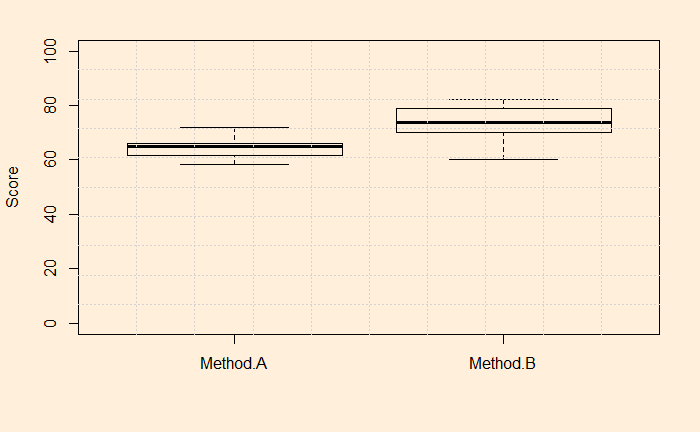
As done before, we plot the data first; we use a box plot.
2-Sample t-test
The R code for the 2-sample t-test is the same (“t.test”) as before, but you need to input both sets of data in it.
	Two Sample t-test

data:  AB_data$Method.A and AB_data$Method.B
t = -4.2402, df = 28, p-value = 0.00022
alternative hypothesis: true difference in means is not equal to 0
95 percent confidence interval:
 -13.357755  -4.655578
sample estimates:
mean of x mean of y
 64.05733  73.06400
Before jumping to the answers, you may have noticed that I have used var.equal = TRUE here. In other words, I have assumed the variances of each group to be equal; well, more or less similar! Depending on the variances, there are two methods: the standard method is used when the variances are similar. When they are different, we need to use the Welch t-test. Let’s check the standard deviations of the groups. They are 3.86 and 7.27.
We’ll make no assumptions here, and I repeat the calculations using var.equal = FALSE. Here are the results.
	Welch Two Sample t-test

data:  AB_data$Method.A and AB_data$Method.B
t = -4.2402, df = 21.308, p-value = 0.0003561
alternative hypothesis: true difference in means is not equal to 0
95 percent confidence interval:
 -13.42015  -4.59318
sample estimates:
mean of x mean of y
 64.05733  73.06400
Similar answers suggest that variances are, indeed, close to each other.
Interpreting results
We will start with the p-value now. p = 0.0003561, which is less than the standard significance level of 0.05. Therefore, we can reject the null hypothesis. i.e., the sample data suggest that the population means are different.
The 90% confidence interval [-13.4, -4.6] escapes zero, which is no more a surprise and reinforces the fact that the null hypothesis, zero difference between the means, is not valid here. The negative sign on the difference only means that the mean of method A is lower than method B.
In the previous post, we have done a 1-sample t-test on students’ scores to check for statistically significant changes from the past year’s average. Today we will spend time interpreting the results. First, the results:
One Sample t-test
data: test_data$score
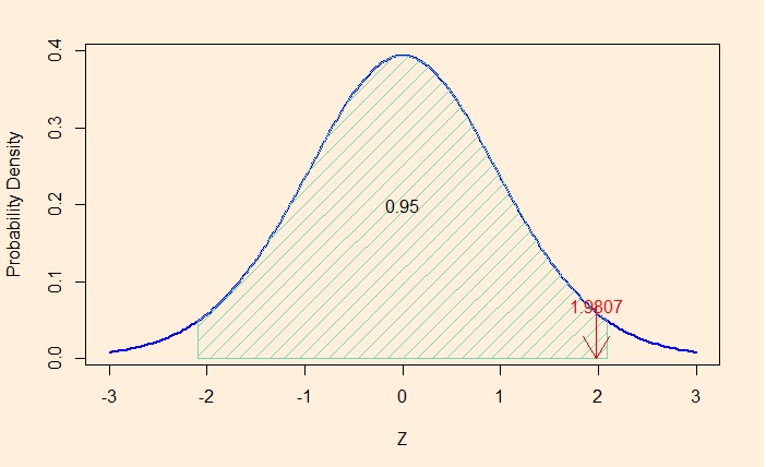
t = 1.9807, df = 19, p-value = 0.06229
alternative hypothesis: true mean is not equal to 50
95 percent confidence interval:
49.80912 56.92088
sample estimates:
mean of x
53.365
Since there were 20 data points in the study, the degree of freedom (df) is 19. The sample mean is 53.365, which is higher than the reference value of 50; however, the calculated t-value is 1.9807. If you choose alpha (the significance level) to be 0.05 (5%), the t-value should be more than 2.09 to reject the null hypothesis. In other words, 1.9807 is within the 95% confidence area (of the t-distribution).
Remember that not being able to reject the null hypothesis doesn’t mean that you accept the null hypothesis. In simple terms, there is no way to say that the population mean for this year remained at 50. The 95% confidence interval tells you that the actual population mean is between 49.80912 and 56.92088, i.e., the range includes the reference value (50).
Of course, it also doesn’t mean that the sample mean of 53.365 is the new population mean!
Finally, the dear old p-value: the p-value is more than 0.05, which is the standard significance level we chose in the analysis. It is 0.06229.
We will do a 1-sample t-test from start to finish using R. You know about the t-test, and we have done it before.
What is a 1-sample t-test?
It is a statistical way of comparing the mean of a sample dataset with a reference value of the population. The reference value (reference mean) becomes the null hypothesis and what we do in the t-test is nothing but hypothesis testing.
Assumptions
There are a few key assumptions that we make before applying the test. First, it has to be a random sample. In other words, it has to be representative; otherwise, it would not provide any valid inference for the population. The second condition requires that the data must be continuous. Finally, the data should follow a normal distribution or have more than 20 observations.
Example
You have done a major revamp of the school curriculum this year. You know the state-level average test score last year was 50. You like to find out whether the average score this year is different from the previous. So, you conducted a random sample of 20 participants, and their scores are below:
Student
Score
1
40.5
2
50.1
3
60.2
4
51.3
5
42.1
6
57.2
7
37.9
8
47.2
9
58.3
10
60
11
61.2
12
52.5
13
66
14
55
15
58
16
55.1
17
47.4
18
52.1
19
63.1
20
52.1
mean = 53.365
Is that significant?
The mean = 53.365 suggests there was an improvement in students’ scores. But that is a quick conclusion; after all, we took only a sample, which will have variability, and, unlike the population mean, the sample means will follow a distribution. So we will do testing the following hypotheses:
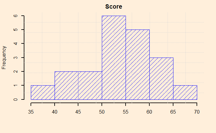
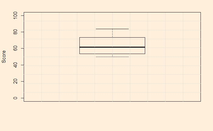
The null hypothesis, N0: The mean of the population this year is 50 The alternative hypothesis, NA: The mean of the population this year is not 50 But, before that, let’s plot the data. It is a good habit that can already give a feel of the data quality, scatter, outliers etc.
The data look pretty ok, with no outliers, reasonably distributed etc. Now, the t-test. It’s simple: use the R function, t.test (stats package), and you get everything.
	One Sample t-test

data:  test_data$score
t = 1.9807, df = 19, p-value = 0.06229
alternative hypothesis: true mean is not equal to 50
95 percent confidence interval:
 49.80912 56.92088
sample estimates:
mean of x
   53.365
We shall see the inferences of this analysis in the next post.
Michael Radelet’s study in 1981 is an example of ecological fallacy but, more importantly, exposed the racial disparity that existed in the process of ensuring criminal justice in the US.
Radelet collected data from 20 counties of Florida indictments of murders that occurred in 1976 and 1977. His research team have identified 788 homicide cases, and after cleanup of incomplete information, 637 remained for further investigation.
Ecology
Let us start with the overall results: the race composition of the death penalty is 5.1% (17 death penalties out of a total of 335 defendants) for blacks and 7.3% (22 out of 302). There is nothing much in it, or if you are right-leaning with a bit of vested interest, you might even say the judges are more likely to hand death penalties to the whites!
The details
Now, what happens to justice if the victims were white? If the person died in the case was white, there is a 16.7% chance for the black defendants to get a death sentence vs 7.7% for a white. On the other hand, if the person murdered was back, the percentages are 2.2 for blacks and 0 for whites. Black lives were priced lower, and whites seemed to have some birth rights to take out some of it!
The complete dataset is below; you may do the math yourself.
# Cases
First degree indictments
Sentenced to Death
Non-Primary White victim
Black defendant
63
58
11
White defendant
151
124
19
Non-Primary Black victim
Black defendant
103
56
6
White defendant
9
4
0
Primary White victim
Black defendant
3
1
0
White defendant
134
73
3
Primary Black victim
Black defendant
166
51
0
White defendant
8
4
0
Total
637
371
39
Radelet, M.L.; Racial Characteristics and the Imposition of the Death Penalty, American Sociological Review, 1981, 46 (6), 918-927
A lot of data we know describe the general trends of a region or group than from its members. E.g. the crime rate of a city is estimated based on the total number of crimes divided by the number of people. It is not calculated based on surveys of every individual member. A city can be high in crime rates, yet 99% of the individuals are not under any threat to their life or property. In other words, there may be a few pockets in the city that experience disproportionately more crimes than the rest.
Ecological fallacy describes the logical error when we take a statistic meant to represent an area or group and apply it to the individuals or objects inside. It gets the name because the data was meant to describe the system, the environment or the ecology.
A lot of stereotypes arise out of ecological fallacy. A well-known example is racial profiling, in which a person is discriminated against or stereotyped against her ethnicity, religion or nationality. Simpson’s paradox, something we had discussed in the past, is a special case of ecological fallacy.
A classical case was the 1950 paper published by Robinson in American Sociological Review. He found a positive correlation between migrants (colour) and illiteracy. Yet, he found, at the state level, a negative correlation (-0.53) between illiteracy and the number of people born outside the US. This was counterintuitive. One possible explanation is that while migrants tend to be more illiterate, they tend to migrate to regions that are, on average, more literate, such as big cities.
We have seen the p-value before. A higher p-value of a test suggests that the sample results are consistent with the null hypothesis. Correspondingly, to reject the null hypothesis, you like to have lower p-values.
p-values are probabilities observing this extreme sample statistics when the null hypothesis is correct. For example, if 0.05 is the p-value of a study to test the effectiveness of a drug, then you should understand that even if the medicine has no effect, 5% of the studies will give the results you obtained.
It doesn’t stop here. People now think that 5% is the error rate of the test. And this is termed the p-value fallacy. The error associated with a particular p-value is estimated to be much higher than the p-value.