Decision Making

The Ultimatum Game – The Game Theory Version

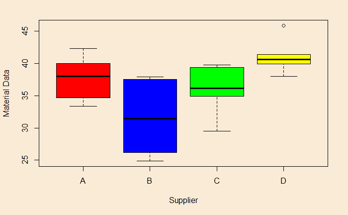
We have seen what behavioural scientists had observed when carrying out the ultimatum game on their subjects. Ultimatum game also has an economic side theorised by the game theorists for the rational decision-maker. A representation of the game is below.

Unlike the simultaneous games we had seen before, where we used payoff matrices, this is a sequential game, i.e. the second person starts after the first one has made her move. The first type is a normal form game and is very static. The one shown in the tree above is an example of an extensive form game.

The game

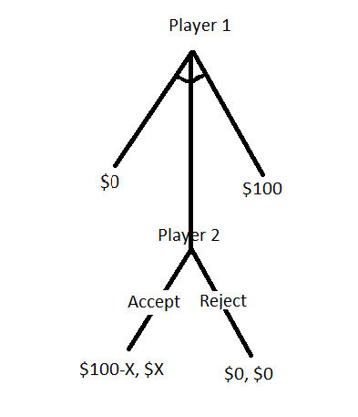
Player A has ten dollars that she splits between her and player B. In the game design, A has to make the proposal and B can accept or reject it. If B accepts the offer, both the players get the money per the division proposed by A. If B refuses, no one gets anything.

Backward induction

Although player A starts the game by spitting 10 dollars between herself and player B, her decision gets influenced by what she assumes about B’s decision (accept/reject). In other words, A requires to begin from the ending and work backwards. Suppose player A does an unfair split 9-1 in favour of A. B can accept the 1 dollar or get nothing by rejecting. Since one is better than zero, B will probably take the offer. If A makes a fair split, then also B will accept the 5. That means B will take the offer no matter what A proposes. So player A may choose the unfair path. This is a Nash equilibrium.

What happens if player B makes a threat of rejecting the unfair offer. It may not be explicit; it could just be a feeling in A’s mind. In either case, player A believes in that and thus makes a fair division. And this is what Kahneman learned from his experiments. In-game theory language, the threat from B is known as an incredible threat as it makes no economic sense to refuse even the unfair offer (as 1 > 0)!

References

Games in the Normal Form: Nolan McCarty and Adam Meirowitz

Extensive Form Games: Nolan McCarty and Adam Meirowitz

The Ultimatum Game – The Game Theory Version Read More »

Tukey’s Method Continued

Here are the sampling results of a product from four suppliers, A, B, C and D (Data courtesy: https://statisticsbyjim.com/).

ABCD
40 37.9 36 38
36.9 26.2 39.4 40.8
33.4 24.936.3 45.9
42.3 30.3 29.5 40.4
39.1 32.6 34.9 39.9
34.737.539.841.4

Hypotheses

N0 – All means are equal
NA – Not all means are equal

Input the data

PO_data <- read.csv("./Anova_Tukey.csv")
as_tibble(PO_data)

Leads to the output (first ten entries)

Material Strength
<chr>     <dbl>
B	  37.9			
C	  36.0			
D	  38.0			
A	  40.0			
A	  36.9			
C	  39.4			
A	  33.4			
B	  26.2			
B	  24.9			
B	  30.3

Plot the data

par(bg = "antiquewhite")
colors = c("red","blue","green", "yellow")
boxplot(PO_data$Strength ~ factor(PO_data$Material), xlab = "Supplier", ylab = "Material Data", col = colors)

F-test for ANOVA

str.aov <- aov(Strength ~ factor(Material), data = PO_data)
summary(str.aov)

Output:

                 Df Sum Sq Mean Sq F value Pr(>F)   
factor(Material)  3  281.7    93.9   6.018 0.0043 **
Residuals        20  312.1    15.6                  
---
Signif. codes:  0 ‘***’ 0.001 ‘**’ 0.01 ‘*’ 0.05 ‘.’ 0.1 ‘ ’ 1

Reject null hypothesis

We at least reject the null hypothesis because the p-value < 0.05 (the chosen significance level). The F-value is 6.018. Another way of coming the conclusions is to find out the critical F value for the degrees of freedoms, df1 = 3 and df2 = 20.

qf(0.05, 3,20, lower.tail=FALSE)
pf(6.018, 3, 20, lower.tail = FALSE)

Lead to

3.098391      # F-critical
0.004296141   # p-value for F = 6.018

Tukey’s test for multiple comparisons of means

TukeyHSD(str.aov)
Tukey multiple comparisons of means
    95% family-wise confidence level

Fit: aov(formula = Strength ~ factor(Material), data = PO_data)

$`factor(Material)`
         diff        lwr        upr     p adj
B-A -6.166667 -12.549922  0.2165887 0.0606073
C-A -1.750000  -8.133255  4.6332553 0.8681473
D-A  3.333333  -3.049922  9.7165887 0.4778932
C-B  4.416667  -1.966589 10.7999220 0.2449843
D-B  9.500000   3.116745 15.8832553 0.0024804
D-C  5.083333  -1.299922 11.4665887 0.1495298

Interpreting pair-wise differences

You can see that the D-B difference, 9.5, is statistically significant at an adjusted p-value of 0.0022. And, as expected, the 95% confidence interval for D-B doesn’t include 0 (no difference between D and B).

By the way, the message, the difference between blue box and yellow, was already apparent had you paid attention to the box plots we made in the beginning.

Reference

Hypothesis Testing: An Intuitive Guide: Jim Frost

Tukey’s Method Continued Read More »

Tukey’s Method: Who Made the Difference?

In the previous ANOVA exercises, we found that data suggested rejecting the null hypothesis. To remind you of the two hypotheses,
N0 – All means are equal
NA – Not all means are equal
So, we at least rejected the proposition that all means are equal because the p-value was lower than the chosen significance level of 0.05 (or the F value was outside the critical F value corresponding to the 0.05 level). But we have no idea which of the pairs of means had the most significant difference.

Tukey method can create confidence intervals for all pair-wise differences while controlling the family error rate to whatever we specify.

Family error rate

You know what is an error rate. It is the probability that the null hypothesis is correct when you reject it when the p-value is less than the significance level. At a significance level is 0.05, there is a 5% chance of getting your outcome when the null hypothesis is correct. The situation is called a false positive.

The p-value we obtained for the material testing problem was 0.03, but it was for the entire family of four vendor groups (each with ten samples). This is the experiment-wise or family-wise error rate. Since our significance level for the F-test was kept at 0.05, we can regard the family error rate to be 5%.

Four groups, six comparisons

Since we had four groups (factors) of samples, each representing one vendor, we have six possible comparisons. They are:

#Comparison
1Vendor 2-Vendor 1
2Vendor 3-Vendor 1
3Vendor 4-Vendor 1
4Vendor 3-Vendor 2
5Vendor 4-Vendor 2
6Vendor 4-Vendor 3

Family-wise error rate, 0.05, is the grand union of all pair-wise error rates. If the pair-wise error is alpha, family-wise error = (1 – (1-alpha)C), where C is the number of comparisons. If you substitute alpha = 0.05 and C = 4, you get the family-wise error as 0.26. Obviously, 26% is too high a significance level.

Tukey method preserves the family-wise error rate to what we specify, say, 0.05, and therefore the pair-wise error rates could be about 0.0085.

By keeping all these points in mind, let’s perform the Tukey’s method on our dataset using R.

TukeyHSD(res.aov)

Which leads to the following output:

Tukey multiple comparisons of means
    95% family-wise confidence level

Fit: aov(formula = Strength ~ factor(Sample), data = AN_data)

$`factor(Sample)`
                         diff        lwr       upr     p adj
Vendor 2-Vendor 1 -2.26479763 -4.7917948 0.2621995 0.0924842
Vendor 3-Vendor 1 -0.51997359 -3.0469707 2.0070236 0.9448076
Vendor 4-Vendor 1 -2.36456760 -4.8915647 0.1624295 0.0736423
Vendor 3-Vendor 2  1.74482404 -0.7821731 4.2718212 0.2632257
Vendor 4-Vendor 2 -0.09976996 -2.6267671 2.4272272 0.9995613
Vendor 4-Vendor 3 -1.84459400 -4.3715911 0.6824031 0.2197059

In the next post, we will do a complete exercise of ANOVA including the Post Hoc test.

Hypothesis Testing: An Intuitive Guide: Jim Frost

Tukey’s Method: Who Made the Difference? Read More »

F – Statistics

We have seen how F-statistics work to test the hypotheses in one-way ANOVA. We also know the definition of F as a ratio between two variances. Variances measure how spread the data is around the mean, estimated as the sum of squared deviation divided by the degrees of freedom. If you forgot, you get the standard deviation if you take the square root of the variance.

F = Between groups variance / Within-group variance

F-tests use F-distribution

Recall how we used the t-distribution or binomial distribution to determine the probability where the null hypothesis was true. F-distribution, too, has a characteristic shape and is based on two parameters – the degrees of freedom 1 and 2, the ones used in the numerator and denominator, respectively.

In the case of the material strength problem we have been working out in the past two posts (four groups with ten samples each leading to df1 =4-1 = 3 and df2 = 4 x (10-1) = 36), the F-distribution appear in the following form.

One way to understand the above plot is to imagine you are repeating the sampling several times (keeping for vendors and taking ten samples each so that df1 and df2 remain the same), and the null hypothesis is true. You calculate the F values each time. Finally, if you plot the frequency of those F values, you get a plot similar to the one above.

F – Statistics Read More »

One-way ANOVA – by Hand

Let’s do the ANOVA step by step. We use the F-statistic to accept or reject the null hypothesis by comparing it with the critical F value. Once you get the F-value, you can calculate the p-value based on a significance level.
The definition of F-statistic is

F = Between groups variance / Within-group variance

Between groups variance

Here, you are estimating the variation of the group statistic from the global statistic. In other words, you determine the means of each group and the global mean (of all data or the mean of means). The estimate the difference, square, add up and divide by the degree of freedom like you do standard variance.

Recall the previous example (strength of materials by four vendors). So you have four groups, each containing ten samples. First, estimate four means and the global mean. They are:

VendorVendor 1Vendor 2Vendor 3Vendor 4
Mean11.28.9410.688.84
Samples10101010
Global mean
(= 9.915)
Square for factor10*(11.2-9.915)210*(8.94-9.915)210*(10.68-9.915)210*(8.84-9.915)2
Sum
Square for factor
(= 43.62)
Degrees of freedom
(DF = 4 -1 = 3)

The numerator (mean squares of factor) is calculated by dividing the sum square of factor with the degrees of freedom, i.e., 43.62/3 = 14.54.

Within-group variance

Here, you add up all the variations inside the groups. Add them up and then divide by the sum of the degrees of freedom of each group.

VendorVendor 1Vendor 2Vendor 3Vendor 4
Samples10101010
Degrees of Freedom
(sample – 1)
9999
Within group
Squares for error
(variance x df)
35.81
(3.98 x 9)
79.93
(8.88 x 9)
10.94
(1.22 x 9)
31.78
(3.53 x 9)
Sum
Within group
Squares for error
(= 158.466)
Total
Degrees of Freedom
(= 36)

The denominator (mean squares of error) is calculated by dividing the sum within group squares for error with the total degrees of freedom, i.e., 158.466/36 = 4.402.

F – Statistics = 14.54 / 4.402 = 3.30

The 3.30 is then compared with the critical F-value corresponding to a set significance level, 0.05, in the present case. You can either look up at the F distribution table or use the R function.

qf(0.05, 3,36, lower.tail=FALSE)

The critical value is 2.87. Since the F-statistics in our case is larger than 2.87, we reject the null hypothesis. The p-value turned out to be 0.031.

pf(3.303, 3, 36, lower.tail = FALSE)

One-way ANOVA – by Hand Read More »

One-way ANOVA

We know how to use a 1-sample t-test to perform a hypothesis test on the mean of a single group and a 2-sample t-test to compare two groups. The scope of t-tests ends here as two is the limit. What happens when you have three groups of data? If the number is two or more, you will use the analysis of variance or ANOVA. As we have done before, we will do an ANOVA using R programming.

Comparing four vendors

ANOVA requires an independent variable (categorical factor) and a dependent variable (continuous). The following table will tell you what I meant. The data used in the analysis is taken from https://statisticsbyjim.com/. The strength of certain materials from four vendors is available, and we are determining if there is a statistically significant difference between the mean strengths. Here is how a few selected entries appear (out of 40).

VendorStrength
Vendor 111.71
Vendor 111.981
Vendor 18.043
Vendor 27.77
Vendor 210.74
Vendor 210.72
Vendor 39.65
Vendor 38.79
Vendor 310.86
Vendor 46.97
Vendor 49.16
Vendor 48.67

Note that the categorical factor, vendor names (1, 2, 3 and 4), divided the continuous data into four groups. Before performing ANOVA, we plot the data and check how they look.

par(bg = "antiquewhite")
boxplot(AN_data$Strength ~ factor(AN_data$Vendor), xlab = "Vendor", ylab = "Strength of Material")

The null and alternate hypotheses are:

N0 = four mean strengths are equal
NA = four mean strengths are not equal

Doing ANOVA is pretty easy; the following commands will do the job.

sum_aov <- aov(AN_data$Strength ~ factor(AN_data$Vendor))
summary(sum_aov)
                      Df Sum Sq Mean Sq F value Pr(>F)  
factor(AN_data$Vendor)  3  43.62  14.540   3.303 0.0311 *
Residuals              36 158.47   4.402                 
---
Signif. codes:  0 ‘***’ 0.001 ‘**’ 0.01 ‘*’ 0.05 ‘.’ 0.1 ‘ ’ 1

We are testing the statistical significance by the F-test. And here is the most important thing, the p-value is 0.03, less than the 0.05 we chose. So the null hypothesis is rejected. We will see what they all mean, in the next post.

Hypothesis Testing: An Intuitive Guide: Jim Frost

One-way ANOVA Read More »

The Responsibility Bias

It is a commonly observed phenomenon where people claim more credit for their contributions to collecting activities than they deserve. Examples are partners taking more than 50% credits inside marriage relationships, award-winning personalities resisting giving enough credits to their collaborators etc.

The person I see every day

Responsibility bias does not necessarily emerge out of the evilness of an individual. However, it is exacerbated by their ego – too much focus on themselves. Understandably, the quantity of information that a person has on herself is more than what she has on other people. And if she fails to recognise that fundamental disparity, she is expected to make the mistake of shunning others.

Perspective thinking

Noticing and acknowledging the contribution of others requires deliberate effort. One of the techniques is to deliberately consider the members in the group as individuals, not just the ‘rest of the group’.

This is what Caruso and Bazerman at Harvard observed this phenomenon in their investigations on perspective-taking with academic collaborators. They selected articles with three to six authors from five journals, and questionnaires were sent to the writers asking about their experience with the author group.

The questionnaire was divided into 2: 1) self-focused, in which the receivers were asked to write about their contribution (in percentages), and 2) other-focused, in which the subject was first given a task to write down the names of the co-contributors and then about their contributions, including themselves. As a measure, the participants were asked two questions: 1) how much they enjoyed the work and 2) if they were willing to collaborate on a future publication.

As predicted by the investigators, on average, the self-focused group had allocated a higher responsibility to themselves compared to the other-focused.

References

The costs and benefits of undoing egocentric responsibility assessments in groups: Caruso and Bazerman
Give and Take: Adam Grant

The Responsibility Bias Read More »

The Ultimatum Game – The Kahneman Experiment

In yet another Kahneman experiment, the team tried to play the ultimatum game with a group of psychology and business administration students. If you forgot what the game was, here is the description.

The game

Experiment 1

In their experiment, player A got paired with player B at random. There were several pairs. Each duo got $10 that could be divided between the two as proposed by one of the pairs. If player A allocated the division and was acceptable to player B, the payoffs were done accordingly. If the proposed division was unacceptable to player B, neither got anything.

Much to the surprise, because it violated the standard game theory prediction, the researchers found that the majority (75%) of the participants split the offers equally. There were also rejections of some of the proposals.

Experiment 2

The experiment had two parts. The first part was the ultimatum game with a few differences. The subjects only got two possibilities to divide $20: 18:2 or 10:10. And the receiver had no option to reject. In the second part, the participants were matched with two others. She then got a chance to split $12 evenly between herself and the person (the unfair one) who gave away $2 in the previous game (if one of them happened to be in the match) or to split $10 evenly with the even-splitters (the fair ones) of the earlier part.

76% of the people split evenly in the first part of the experiment. In the second part, there was a clear preference (74%) to punish the unfair allocators even when that would mean a $1 cost to the allocator.

The Ultimatum Game – The Kahneman Experiment Read More »

The Ultimatum Game

Adam Grant, in his best-selling book Give and Take, describes the behavioural characteristics of three types of humans based on their attitudes towards other people – takers, matchers and givers. According to the author, takers give away (money, service or information) when the benefits to themselves are far more than the personal costs that come with the transfer. Givers, on the other extreme, relish the value to others more than the personal cost to themselves. Naturally, the matchers are in between – strictly reciprocating.

Grant reference to a paper published by Kahneman et al. in 1986 based on a concept called the ultimatum game, a well-known idea in game theory. Today, we will look at the game. We’ll discuss the study results another day.

The game

We will illustrate the concept through a 100-dollar game. Player 1 (donor) gets 100 dollars, and she can offer – anything from 0 to 100 – to player 2 (receiver). If player 2 accepts, she gets it, and player 1 takes the rest (100 – X). If player 2 rejects the offer, then no one gets anything.

Rationality vs sense of fairness

If the receiver was rational, her actions would have been governed by her self-interest, as expected by economic theories, and she would have taken whatever was offered. After all, something is better than nothing. But this doesn’t always happen. There is a limit to the offer below which the receiver may feel the donor’s injustice.

Further Reading

Give and Take: Adam Grant
Ultimatum Games: William Spaniel

The Ultimatum Game Read More »

Newcomb’s Paradox

The paradox was created by William Newcomb and was first published by Robert Nozick in 1969.

Imagine there is a being that has the superpower to predict your choices with high accuracy, and you know that. There are two boxes, B1 and B2. You know that B1 contains 1000 dollars and B2 carries either one million dollars or nothing. You have two choices: 1) take what is inside both the boxes or 2) only take what is in the box B. Further, it is a common knowledge that:
1) If the being predicts that you will take both the boxes, it will not add anything to box B
2) If the being knows you will only take box B, it will add a million dollars to it.

I guess you remember the definition of common knowledge: you know that he knows that you know stuff!

What will you choose?

There are two possible arguments for leading to two different decisions.
1) You know the being will read your mind and put nothing in B if you choose both the boxes and add a million if only B is chosen. So select option 2 (select box B).
2) The being has already made the decision (after reading your mind), and the only way for you to minimise the damage is to select option 1 (select both the boxes).

In polls conducted to understand their preferences, people often tied at 50:50; there are takers for both options. But why is that?

Dominance principle

Let’s first write down the payoff matrix.

The Being
predicts
you take B
The Being
predicts
you take both
You take Box B1 million0
You take both1 million +
1000
1000

The dominance principle states that if you have a strategy that is always better, you make a rational decision to choose that. In this case, that is taking both boxes.

Here is a thought experiment to explain this perspective. Imagine the other side of the box is transparent, and your friend is standing on that side. She can see the amount inside. Although she can’t tell you anything, what would she be hoping for? Well, if she sees that the being had put a million in box B, you would be better off taking that box and the one that carries 1000. If She finds the being did not add anything, she would still like you to take both the boxes to win the guaranteed 1000.

Expected value theory

While the expected utility theory is better suited to describe situations like these, I have gone for the expected value theory as I find it easier to explain things. We estimate the expected value of each action by multiplying the value by its probability. Imagine you trust the being is accurate at 90%, the following two calculations get you the value of your decision, and you choose what gives the highest.

You take B0.9 x 1,000,000 + 0.1 x 0
= 900,000
You take both0.9 x 1000 + 0.1 x 1,001,000
= 101,000

Therefore, you select only box B.

Newcomb’s Problem and Two Principles of Choice: Robert Nozick
Newcomb’s Paradox – What Would You Choose?: Smart by Design

Newcomb’s Paradox Read More »