The confusion of stupidity for irrationality is common but equally a misunderstanding. While being stupid and irrational may lead to the same outcome, poor decision-making, we should realise that the two are distinctly different. Most humans are not stupids; a lot of us are irrational in something or the other.
Stupidity is the error of judgement caused by inherent limitations of intelligence. Irrationality is due to risk illiteracy or the lack of knowledge of probability. One may be mitigated; the other is doubtful.
It is easy to prove your weatherman is wrong. Easier if you are short-term memory and are oblivious to probability.
Imagine you tune into your favourite weather program; the prediction was: a 10% chance of rain today. You know what it means: almost a dry day ahead. The same advice continued for the next ten days. What is the chance there was rain on at least one of those days? The answer is not one in ten, but two in three!
You can’t get the answer by guessing or using common sense. You must know how to evaluate the binomial probability. For instance, to calculate the chance of getting at least one rain in the next ten days, you use the formula and subtract it from one.
Decision making
All these are nice, but how does this forecast affect my decision-making? The decision (take a rain cover or an umbrella) depends on the threats and alternate choices. On a day with a 10% chance of rain predicted, I will need a reason to take an umbrella, whereas, on a day of 90%, I need a stronger one not to take precautions.
Why the weatherman is wrong
Well, she is not wrong with her predictions. But the issue lies with us. Out of those tens days, we may remember only the day it rained because it contradicted her forecast of 10%. And the story will spread.
We have seen the concepts of joint and conditional probabilities as mathematical expressions. Today, we discuss an approach to understanding the concepts using something familiar to us – using tables.
Tabular power
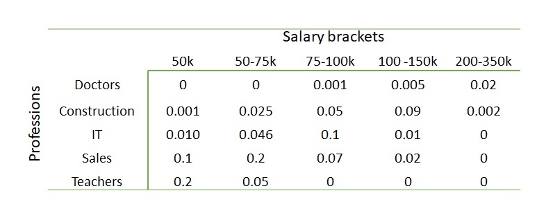
Tables are a common but powerful way of summarising data. Following is one summary from a hypothetical sample collection of salary ranges of five professionals.
It is intuitive for you to know that the values inside the table are the joint occurrences of the row attributes (professions) and column attributes (salary brackets). You get something similar to a probability once you divide these numbers by the total number of samples (= 1000). In other words, the values inside the table give us the joint probabilities.
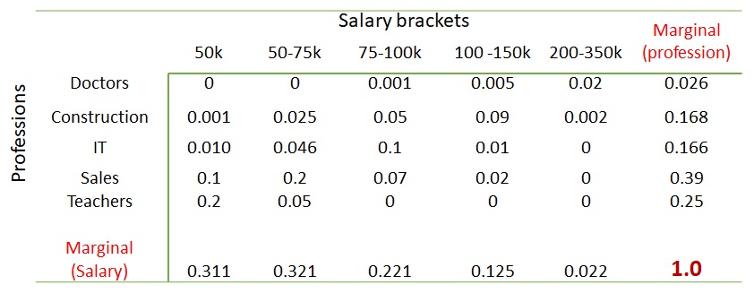
Can you spot the marginal probabilities, say, that of doctors in that sample space? Add the numbers of the rows or columns; you get it.
Conditional probabilities
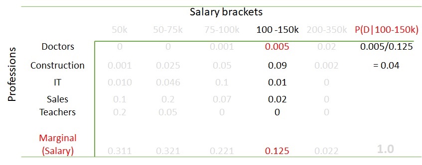
What are the chances it is a doctor if the salary bracket is 100-150k per annum? You only need to look at the column for 100-150k (because that was given) and then calculate the proportion of doctors in it. That is 0.005 out of 0.125 or 0.005/0.125 = 0.04 or 4%.
Look it this way: in the sample space, were 125 people in the given salary bracket, of which five were doctors. If the sample holds it for the population, the percentage becomes 5/125 or 4%.
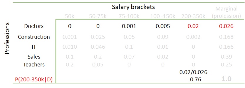
The calculation can also work in the other way. What is the probability of someone in the salary bracket of 200-350k per year, given the person is a doctor? Work out the math, and you get 76%.
A quick recap: in the previous post, we set a target of finding the bias of a coin by flipping it and collecting data. We have assumed a prior probability for the coin bias. Then established a likelihood for a coin that showed a head on a single flip.
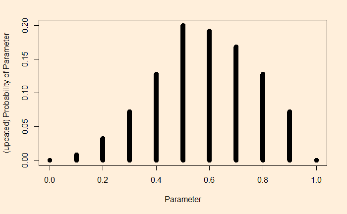
We know we can multiply prior with the likelihood and then divide by the probability of the data.
The outcome (posterior) is below.
Look at the prior and then the posterior. You see how one outcome (heads on one flip) makes a noticeable shift to the right. It is no more equally distributed to the left and the right.
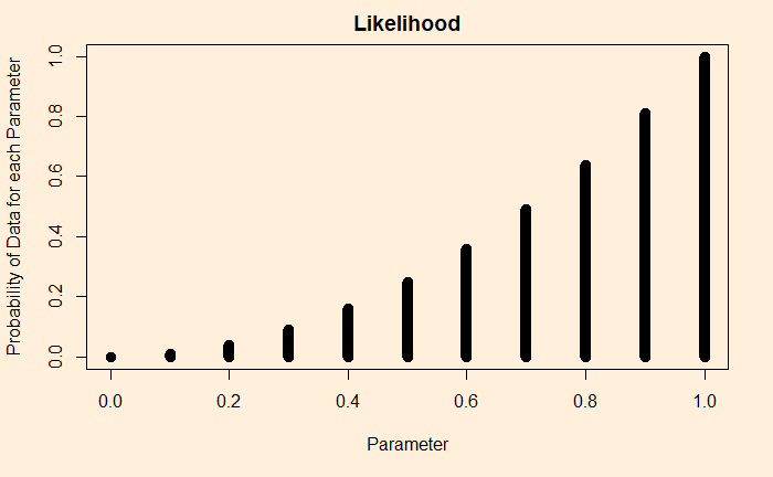
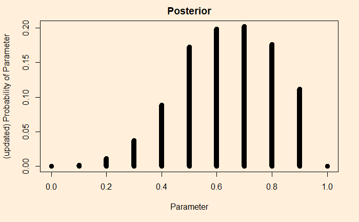
What would happen if, for the same prior, but getting two heads? First, calculate the likelihood:
You can see a clear difference here as the appearances of the two heads changed the likelihood heavily to the right. The same goes for the updated chance (the posterior).
Bayesian inference is a statistical technique to update the probability of a hypothesis using available data with the help of Bayes’ theorem. A long and complicated sentence! We will try to simplify this using an example – finding the bias of a coin.
Let’s first define a few terms. The bias of a coin is the chance of getting the required outcome; in our case, it’s the head. Therefore, for a fair coin, the bias = 0.5. So the objective of experiments is to toss coins and collect the outcomes (denoted by gamma). For simplicity, we give one for every head and zero for every tail.
The next term is the parameter (theta). While the outcomes are only two – head or tail, their tendency to appear can reside on a range of parameters between zero and 1. As we have seen before, theta = 0.5 represents the state of the unbiased coin.
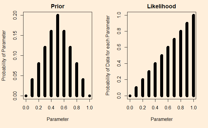
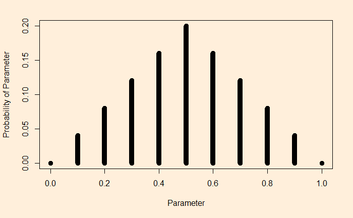
The objective of Bayesian inference is to estimate the parameter or the density distribution of the parameters using data and starting guesses. For example:
In this picture, you can see an assumed probability distribution of coins made from a factory. In a way, this is to say that the factory produces ranges of coins; we think the highest probability to be theta = 0.5, the perfect unbiased coin, although all sorts of other imperfections are possible (theta < 0.5 for tail-biased and theta > 0.5 for head-biased).
The model
It is the mathematical expression for the likelihood function for every possible parameter. For coin tosses, we know we can use the Bernoulli distribution.
If you toss a number of coins, the probability of the set of outcomes becomes:
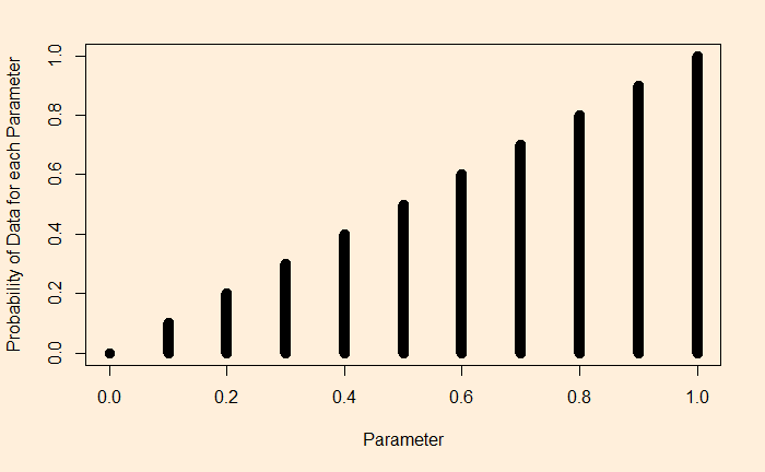
Suppose we flip a coin and get heads. We substitute gamma = 1 for each of the theta values. A plot of this function for the following type appears:
Let’s spend some time understanding this plot. The plot says: if I have a theta = 1, that is a 100% head-biased coin, the likelihood of getting a head on a coin flip is 1. If it is 0.9, then 0.9 etc., until you reach a tail-biased one at theta = 0.
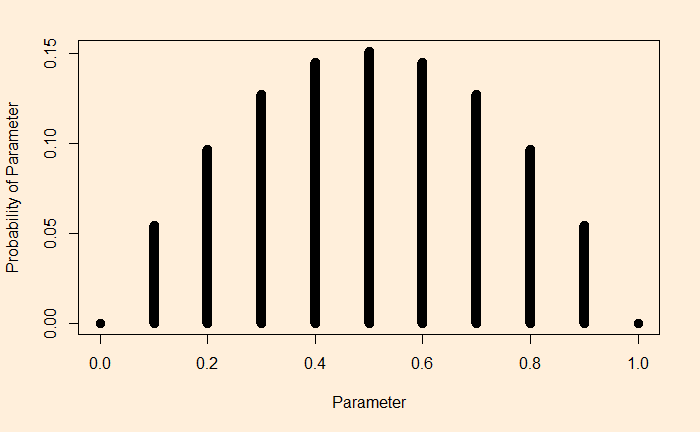
Imagine, I did two flips and got a head and a tail:
The interpretation is straightforward. To take the extreme left point: If it was a tail-biased coin (the parameter, theta = 0), the probability of getting one head and one tail is extremely low. Same for the extreme right (the head-biased).
Posterior from prior and likelihood
We have prior assumptions and the data. We are ready to use Bayes’ rule to get the posterior.
We have seenself-assessment bias before. Self-assessment of intelligence falls closer to this. Many studies have shown this bias affects men and women differently. And this led to the term MHFH or Male Hubris, Female Humility in cognitive psychology. Note that this exists despite countless studies which failed to find any difference in the levels of general intelligence between men and women.
Apart from these so-called Dunning–Kruger effects, cultural stereotypes play a role in this gender bias. For example, there are study results in which the participants rated their fathers as more intelligent than mothers. Asking parents about their children also resulted in similar impressions. You add teachers, media, or the society as a whole, to this mix; the disaster is complete.
Higher self-esteem is also seen as a contributing factor to higher self-estimations. And gender, as a sex or a personality trait, masculine vs feminine, has a role in this.
Today we explore the difference between ‘after’ and ‘from’! Because it concerns a famous fallacy called “Post Hoc Ergo Propter Hoc“. So what does this cool-sounding Latin phrase mean? As per Wikipedia, it means: “after this, therefore because of this”. It is the interpretation that something happens after an event to something from it. Take the example of the CDC’s Vaccine Adverse Event Reporting System (VAERS).
Adverse Event Reporting System
The Centers for Disease Control and Prevention of the United States uses VAERS as a system to monitor adverse events following vaccination. The data was meant for the medical researchers to find patterns and, thereby, potential impacts of vaccines on human health. Naturally, the system gets scores of events ranging from minor health effects to deaths. And a section of the crowd interprets and propagates these events due to vaccination. So, where is the fallacy here?
What happened in 2020
The number of people who died in the US due to heart disease in 2020 is 696,962, which is about 2000 per million population. The figure is 1800 for cancer, 500 for respiratory illness and 310 for diabetes. So, roughly 4610 per million per year due to these four types of diseases.
Thought experiment
Let’s divide 20 million Americans into two hypothetical groups of 10 million each. The first group took the vaccine over one month, and the second did not. What is the expected number of people from the unvaccinated group to die of the four causes mentioned previously? About 3840. But they do not report to the VAERS.
On the other hand, imagine a similar death rate to the vaccinated group. If 10% of those 3840 people report the incident in the system, it will make 384 reports or about 4600 in the whole year.
The first case will be forgotten as fate, whereas the second will be celebrated by the media as: “vaccine kills thousands”!
Probabilistic insurance is a concept introduced by Kahneman and Tversky in their 1979 paper on prospect theory. Here is how it works.
You want to insure a property against damage. After inspecting the premium, you find it difficult to decide to pay for the insurance or leave the property uninsured. Now, you get an offer for a different product that has the following feature:
You spend half the premium but buy probabilistic insurance. In this case, you have a probability p, e.g. 50%, in which you, in case of damage, will pay the rest of the 50% and get fully covered, or the premium is reimbursed, and the damage goes uncovered.
For example, the scheme works in the first mode (pay the reminder and full coverage) on odd days of the month and the second mode (reimbursement and no coverage) on even days!
Intuitively unattractive
When Kahneman and Tversky asked this question to the students of Standford university, an overwhelming majority (80%) was against the insurance. People found it too tricky to leave insurance to luck or chances. But in reality, most insurances are probabilistic, whether you are aware or not. The insurer always leaves certain types of damages outside their scope. The investigators proved using the expected utility theory that probabilistic insurance is more valuable than a regular one.
Tversky, A.; Kahneman, D., Econometrica, 1979, 47(2), 263
We have seen an explanation of the Monty Hall problem of “Let’s make a deal”, using a 100 door-approach. Let’s imagine a 26-door version. You select one, and the host opens 24 doors that do not have the car. Will you switch your choice to the last door standing? The answer is an overwhelming yes.
Now, switch to another game, namely the deal or no deal. The show contains 26 briefcases containing cash values from 0.01 to 1,000,000 dollars. The player selects one box and keeps it aside. Cases are randomly selected and opened to show the cash inside. Periodically, the dealer offers some money to the player to take and quit the game. If the player refuses all offers and reaches the end, she will have to take whatever is in the originally-chosen case.
Monty’s deal or no deal!
Imagine there are just two boxes left – the one you have selected and the one remaining. The remaining cash values are one and one million. Enter Mr Monty Hall and offers a switch. Will you do it? After all, the original recommendation for the case described in the first paragraph was to switch! But here, there is no need to swap, as you have a 50:50 chance of winning a million from your box. Why is that?
Bayes to the rescue
Before I explain the difference, let’s work out the two probabilities using Bayes’ theorem. First, the original one (Let’s make a deal): Let A be the situation wherein your chosen door has the car behind and B the one where 24 gates did not have it.
Substitute the values, P(A) = (1/26), P(A’) = 25/26 and P(B|A) = 1 (the chance of 24 doors have no car given the car is behind your chosen door. Now think carefully, what is P(B|A’), the probability of having no cars behind those 24 doors, given yours does not have a car? The answer is: it remains one because it was the host who opened the door with full knowledge; it was not a random choice!
So, switching increases your chances to 1 – (1/26) = 25/26.
Second, the new one (Deal or no deal version)
As before, P(A) = (1/26), P(A’) = 25/26 and P(B|A) = 1. Here is the twist, P(B|A’) is not 1 because the situation of 24 cases did not produce a million came at random and was not due to your host. The probability of that happening, given your case doesn’t contain the prize, is 1 in 25. So P(B|A’) = (1/25).
Amazing, isn’t it?
Reference
The Monty Hall Problem: The Remarkable Story of Math’s Most Contentious Brain Teaser: Jason Rosenhouse
The trolley problem is a thought experiment in ethics about a scenario in which an onlooker has a chance to save five people being hit by a runaway trolley by diverting it to another track, hitting one person.
The fallacy of dilemma
It is an informal fallacy in which the proponent restricts the options to choose into a few, say, two. It is a fallacy because the framing of the premise is erroneous.
Back to the trolley
In my view, the trolley problem is a false dichotomy (two options) problem that does two things. It forces you to believe that there are only two options – kill five or kill one. It then helps you to justify killing the one as one generous act to save five. And this has been consistently practised by political leaders, especially of the oppressor types, to push their malicious agenda whilst satisfying the collective imagination of the majority.
Dealing with the trolley
The best way to deal is to resist the premise. Why are there diversions or two tracks? Why are there only two tracks? Why is the onlooker not closer to the five so she can save them (by pushing or something)? Why does only the diversion switch work and not the stopping switch?