Let’s revisit the three stores. But there is a slight difference this time.
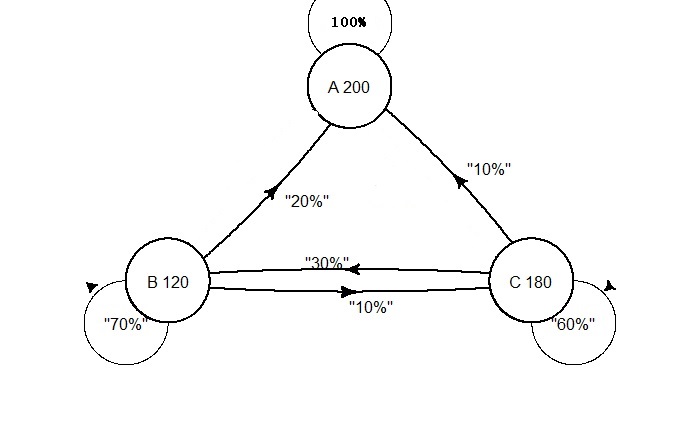
There is no arrow from store A to B or C. The customers who reach A are fully retained or absorbed. This is an absorbing Markov chain. The transition matrix for the above situation is,
You may have guessed it already, but if you continue this chain to develop, the end-state distribution becomes,
A + 0.2B + 0.1 C = A
0 + 0.7B + 0.3 C = B
0 + 0.1B + 0.6 C = C
A + B + C = 1
A + 1.2B + 1.1 C = 1
0 - 0.3B + 0.3 C = 0
0 + 0.1B - 0.4 C = 0
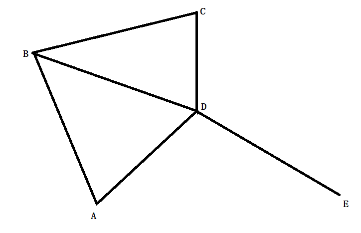
Amy lives in city A and has friends in cities B, C, D, and E. The following scheme represents the direct bus connections to these cities. Every Monday, she takes a direct bus at random, reaches the town, and stays with her friend for a week. How many weeks would she have spent in each city that year if she had done this for a year?
The route map suggests that on a given week, Amy has the following probabilities 1) Equal chances from A to B or D (0.5, 0.5) 2) Equal chances from B to A, C, or D (0.33, 0.33, 33) 3) Equal chances from C to B, D (0.5, 0.5) 4) Equal chances from D to A, B, C or E (0.25, 0.25, 0.25, 0.25) 5) Can move from E to D (1.0)
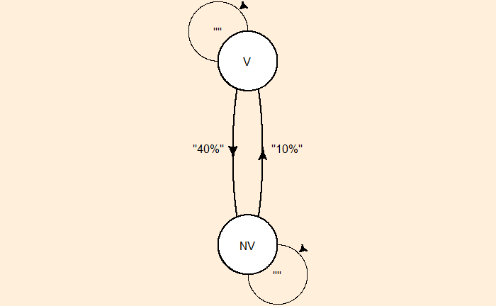
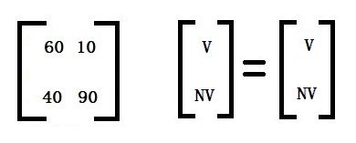
Let’s take another example. For a particular website, 40% of visitors don’t return next time. Of the non-visitors, 10% turn up next time. What is the website’s end-state distribution? Let V represent the visitor and NV the non-visitor.
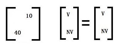
We know the property of the end state: the distribution at which P X* = X*. Let’s fill in the available data.
The columns must add up to 100% or 1.
Let’s now expand the equation and change percentage data to fractions.
0.6 V + 0.1 NV = V 0.4 V + 0.9 NV = NV
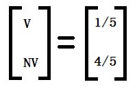
NV = 4 V But we know V + NV must be 1 V + 4 V = 1 V = 1/5 NV = 4/5
It would be interesting to see how the probability matrix is transformed as the number of stages progresses. Here is the original matrix (P), followed by (P10).
0.8  0.2  0.1
0.1  0.7  0.3
0.1  0.1  0.6
0.45 0.45 0.45
0.35 0.35 0.35
0.20 0.20 0.20
Elements in each raw are similar in magnitude, which suggests why the end result after multiplying it with the original proportion is the same after each stage.
Another interesting fact is how Xn changes with the initial proportion, X0. We use the following X0 values. Note that the sum of the proportions must add to 1.
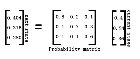
Last time, we saw how the next stage is developed from the current stage using the probability matrix.
X1 = P X0
There is a reason why it is called the Markov chain. The system we have developed can now predict the stage after the next stage, i.e., X2. Multiply the probability matrix with X1.
X2 = P X1
Substituting for X1, X2 = P P X0 X2 = P2 X0 or in general Xn = Pn X0
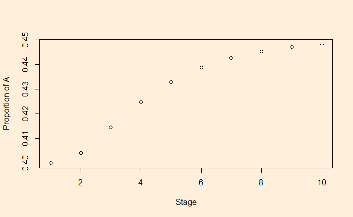
Let’s work out the stage after 10 moves and plot and see where A ends up.
In the last post, we started an example to demonstrate the objective of Markov processes.
The question is, what is the expected number of customers in shops A, B, and C in the following week?
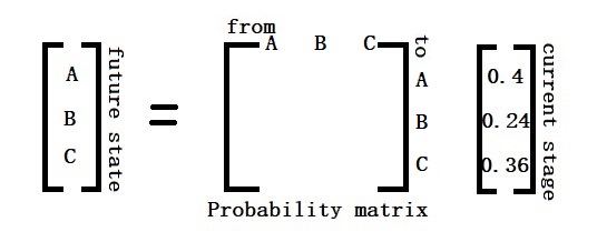
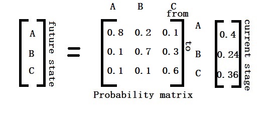
The whole formulation is nothing but future state = present state x a probability matrix. The probability matrix, fundamental to making this translation, is developed from the diagram we created earlier.
The first row of the matrix are the probabilities: A to A, B to A and C to A The second row: A to B, B to B and C to B The third row: A to C, B to C and C to C
Perform the matrix multiplication between the two. Here are the R codes.
The Markov approach is a concept for predicting stochastic processes. It models a sequence in which the probability of the following (n+1) event depends only on the state of the previous (n) event. Therefore, it is also called a ‘memoryless’ process.
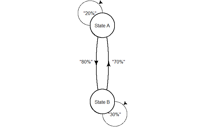
Before performing calculations, let’s familiarise ourselves with the concept and notations. Suppose there are two states: state A and state B. The process is expected to stay in the same stage for 20% of the time and can move to stage B in the remaining 80%. On the other hand, stage B has a 30% chance of staying and a 70% chance of moving to stage A. The following diagram depicts the process.
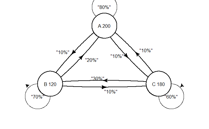
For example, imagine three shops in town—A, B, and C—that attract 200, 120, and 180 customers, respectively, this week. The following possibilities are expected for next week.
Shop A: 80% of the customers stay loyal 10% can move shop B 10% can move shop C
Shop B: 70% of the customers stay loyal 20% can move shop A 10% can move shop C
Shop C: 60% of the customers stay loyal 10% can move shop A 30% can move shop B
The question is, what is the expected number of customers in shops A, B, and C in the following week?
An evil mathematician catches Annie and Ben, putting them in two separate cells. Annie can see 12 trees outside her cell, and Ben can see 8. They are told that together, they can see all the trees, and no tree is seen by both. Every morning, evil comes to each of them and asks if they think there are 18 or 20 trees in total. They can answer or pass. If the answer to either is wrong, they both will be in prison forever. On the other hand, if one of them answers, both will be freed. The questions are asked separately, and Annie and Ben can’t communicate. Can they escape?
Day 1: Had Annie seen 19 or 20 trees, she would have answered 20 to the evil. Since Annie sees only 12 trees, she passes. She also knows Ben sees 6 or 8.
Since the question comes to Ben, who sees 8 trees, he knows that Annie sees 10 or 12 trees. He passes.
Day 2: Annie knows Ben did not answer yesterday, so the question returned on day 2. She also knows that Ben knows she has seen 10 or 12. She thinks if Ben had seen 6, he would have added 12 + 6 = 18 and given the number 18 as the answer. This is because 10 + 6 = 16 is not among the choices. So, she concludes, Ben sees 8 trees. She answers 20 to the evil.
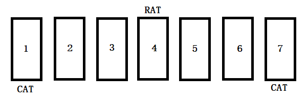
There are seven doors, and a mouse is at door 4. Two cats are waiting at door 1 and door 7. The rat moves one door in a day—either to the left or to the right. When it reaches the cat door, it gets eaten by the cat. What is the average number of days before the rat gets caught?
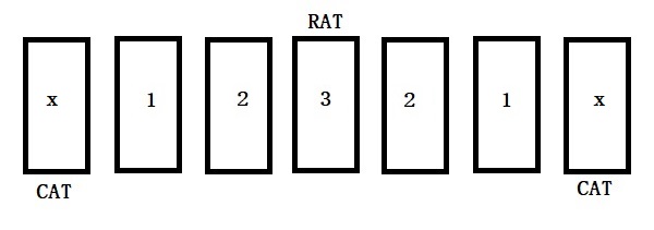
We can rename the arrangement since the mouse sits in the middle of the door sequence.
In the beginning, the mouse is at door 3, and let e3 be the expected time until the mouse gets caught by the cat. After one day, the mouse has a 50% chance of reaching the left or a 50% chance of reaching the right door. Either way, it reaches door 2 and lets e2 be the expected time until caught. Therefore,
e3 = 1 + e2
When the rat is one 2, after one day, the mouse has a 50% chance of reaching door 3 (waiting time e3) or a 50% chance of reaching door 1 (waiting time e1).
e2 = 1 + 0.5 e3 + 0.5 e1
From there, it either reaches door 2 or gets caught in a day.
e1 = 1 + 0.5 e2
Now, we have three linear equations to solve. e3 = 1 + e2 e2 = 1 + 0.5 e3 + 0.5 e1 e1 = 1 + 0.5 e2
Amy walks into a raffle house and finds it about to close. They are raffling off an object with a value of $1000. She finds that only 200 tickets have been sold. Knowing they will draw the winner at any time, how many tickets should Amy purchase to maximise the expected value? The cost is $1 per ticket.
The expected payoff = expected value of the lottery – the price you paid. = value of the object x the probability of winning – the price you paid. the probability of winning = # ticket you bought / total # tickets sold.
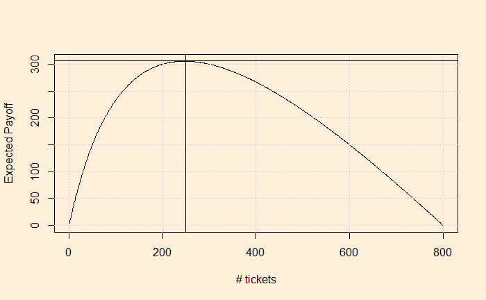
If x is the number of tickets Amy purchased, The expected payoff = [1000 * x /(200 + x)] – x
So, we need to find the x that maximises the payoff. One way to determine is to plot the expected payoff ([1000 * x /(200 + x)] – x) as a function of the # tickets (x) you purchased and see where it maximises.
The number of tickets that maximises the expected payoff is somewhere close to 250.