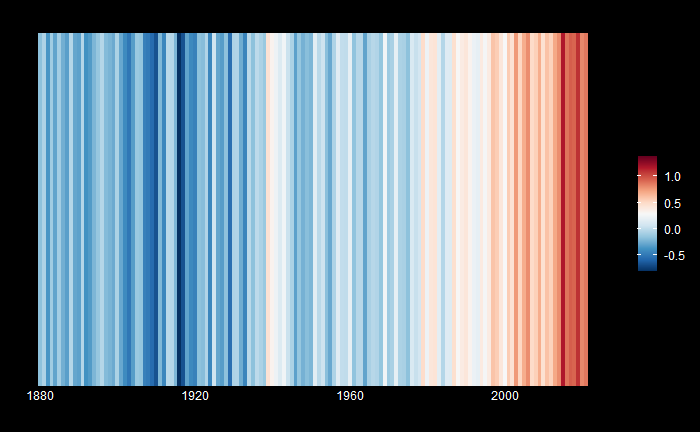
Temperature Anomaly – Warming Stripes
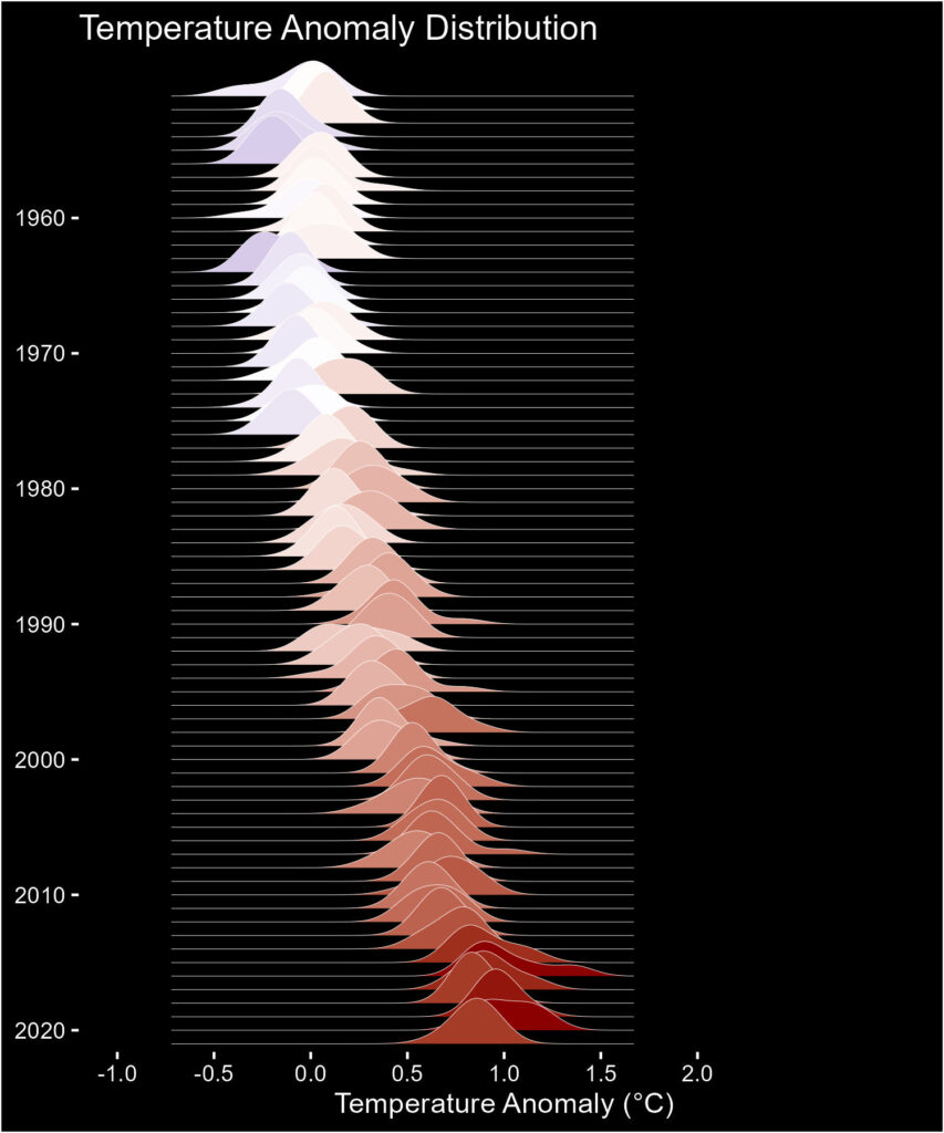
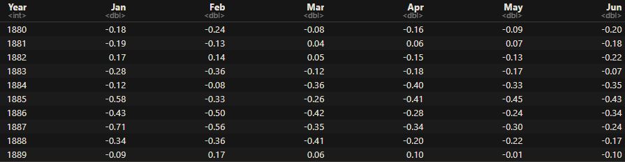
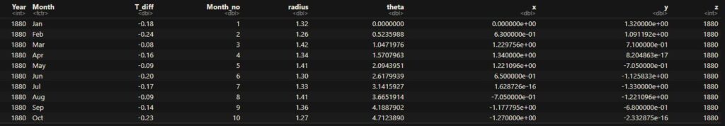
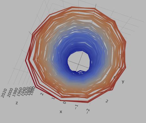
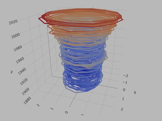
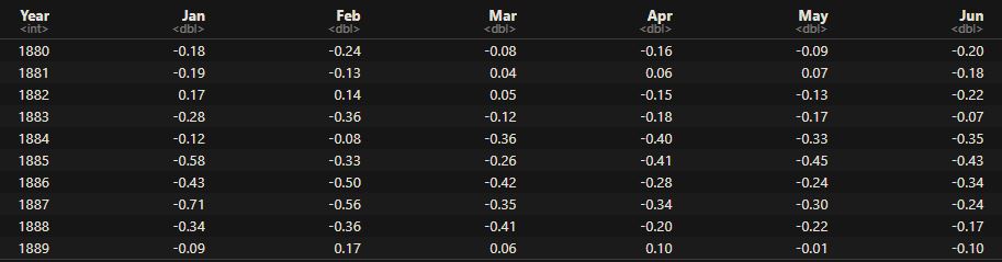
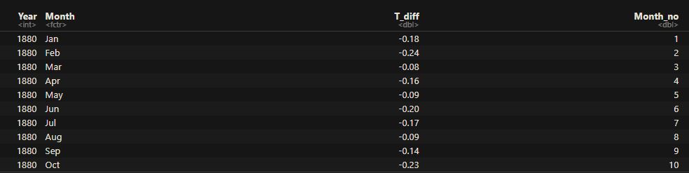
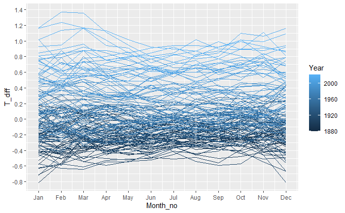
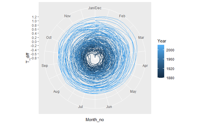
We have seen the spiral plot and ridgeline plot visualising the temperature anomaly (compared to the 1961-80 average). Today, we make another fancy plot – Warming Stripes – using R (again, courtesy: Ed Hawkins of the University of Reading). The data used here is the same as that we described in an earlier post.
c_data %>% ggplot(aes(x = Year, y = 1, fill = T_diff)) +
geom_tile()+
scale_y_continuous(expand = c(0, 0)) +
            scale_fill_gradientn(colors = rev(brewer.pal(11, "RdBu")))+
            guides(fill = guide_colorbar(barwidth = 1))+
            labs(title = "",
            caption = "")+
            theme_minimal() +
            theme(axis.text.y = element_blank(),
                       axis.line.y = element_blank(),
                       axis.title = element_blank(),
                       panel.grid.major = element_blank(),
                       legend.title = element_blank(),
                       axis.text.x = element_text(vjust = 3),
                       panel.grid.minor = element_blank(),
                       plot.title = element_text(size = 14, face = "bold"),
                       panel.background = element_rect(fill = "black"),
                       plot.background = element_rect(fill = "black"),
                       axis.text = element_text(color = "white"),
                       legend.text = element_text(color = "white")
                       )
Temperature Anomaly – Warming Stripes Read More »