Decision Making

Three Prisoners

A, B and C are jailed for a serious crime. They are in separate cells. They came to know that one of them would be hanged the next day, and the other two would be free, based on a lottery. A learns that the lot was already drawn and asks the jailer if he is the unlucky one. The jailer won’t tell that but can give one name other than A, who will be free. Does A benefit from the information?

The sample space for release pairs is AB, AC, and BC, each carrying 1/3 probability.  The probability that A is released is 2 out of these 3 = 2/3. 

When A asks the question, the following scenarios can happen from the warden’s perspective with the respective probabilities. 

1. A and B are released, but the warden says B. The probability is 1/3 x 1. The first part is the probability of AB, and the second part is naming B, as the warden can’t say A’s name.
2. A and C are released, but the warden says C. The probability is 1/3 x 1
3. B and C are released, but the warden says B. The probability is 1/3 x 1/2
4. B and C are released, but the warden says C. The probability is 1/3 x 1/2

Here, there are two scenarios where the warden can say B (1 and 3). Only one involves A. Therefore, given the warden says B, the probability for A to be free is case 1/(case 1+ case 3) = 1/3 / (1/3 + 1/6) = 2/3. A gets no benefit from asking for the name. 
Three Prisoners Read More »

The Happiness Formula – Money Matters

The studies on the correlation between income and happiness have a bit of history. In 2010, a study led by Daniel Kahneman found that the happiness of individuals increases with (log) income until about $75,000 per year and then flattens out. However, the work of Killingsworth (2021) showed contradictory results where happiness just followed a linear trend with the log (income).

Join forces!

The original study of Kahneman and Deaton had survey responses from about 450,000 US residents that captured answers on their well-being.

Killingsworth’s work, on the other hand, had 1,725,994 reports of well-being from 33,391 employed adults (ages 18 to 65) living in the US. It found happiness advancing linearly even beyond $200,000 per year.

The conflict prompted an ‘adversarial collaboration‘ with Barbara Mellers as the facilitator.

The hypothesis

They started with a hypothesis for the test:
1) There is an unhappy minority whose unhappiness reduces with income up to a threshold, then shows no further progress.
2) A happier majority whose happiness continues to rise with income.

The ‘joint team’ stratified Killingsworth’s data into percentiles and here is what they found:

Percentile of
happiness
Slope up to $100kSlope above $100k
5% (least happy)2.340.25
10%1.750.52
15%1.900.34
20%1.840.62
25%1.521.12
30%1.331.21
35%1.261.21

References

Matthew Killingsworth; Daniel Kahneman; Barbara Mellers, “Income and emotional well-being: A conflict resolved”, PNAS, 2023, 120(10).

Daniel Kahneman; Angus Deaton, “High income improves evaluation of life but not emotional well-being”, PNAS, 2010, 107(38).

Matthew Killingsworth, “Experienced well-being rises with income, even above $75,000 per year”, PNAS, 2021, 118(4).

The Happiness Formula – Money Matters Read More »

The fallacy of Hindsight and FOMO

The fallacy of hindsight – the feeling that the fact was evident after the outcome is known – is a significant factor that undermines the truth of probability and risk in decision-making. The occurrences of hindsight bias, or the ‘I knew it’ moments, are prominent when the results are adverse. As per scientists Neal Roese and Kathleen Vohs, there are three bias levels. They are:

  1. Memory distortion (not remembering the earlier opinion)
  2. Inevitability (the event was inevitable)
  3. Foreseeability (the conviction that the person knew it beforehand)

When hindsight bias is all about dismissing the past decision-making process after a negative result, the ‘fear of missing out’ (FOMO) is the intrinsic motivation to act due to (the memories) positive outcomes of the past. Although the term FOMO was initially introduced (in 2004) to describe people’s compulsive behaviour on social networking sites, it is pervasive in several walks of life, including decision-making, investing, and trading, to name a few.

Issues of hindsight bias

The biggest concern is that it discounts the role of probabilities and trade-offs in decision-making, leading to labelling the initial decision-makers as a joke. If you recall the expected value theory, it is almost like forgetting about the probability of failure of the equation. It is more dangerous than just finger-pointing. Hindsight bias causes overconfidence in individuals and decreases rational thinking while navigating complex problems. ‘Always feeling wise’ also reduces one’s ability to learn from mistakes.

And the FOMO

FOMO is just the opposite of what a value investor may want to do. Typically, FOMO leads to chasing stocks during a bull run of the market, or perhaps the very reason for the bull market! While a few lucky ones may be able to cash during the market run, most people with ‘buying high’ end up losing on the crash. FOMO can create collective anxiety in organisations about missing investment opportunities, especially with speculations about the possibilities of ‘things’ happening elsewhere.

References

Hindsight bias: Wiki

Fear of missing out: Wiki

The fallacy of Hindsight and FOMO Read More »

Friedman test

Let’s work out another non-parametric hypothesis test – analogous to repeated measures ANOVA, the Friedman test. The way it works is exemplified by analysing ten runners who participated in a training program. The following are the measured heart rates at regular intervals. Your task is to inspect if there is a significant difference in the heart rate of patients across the three time points.

H_Rate <-  matrix(c(150, 143, 142,
                  140, 143, 140,
                  160, 158, 165,
                  145, 140, 138,
                  138, 130, 128,
                  122, 120, 125,
                  132, 131, 128,
                  152, 155, 150,
                  145, 140, 140,
                  140, 137, 135),
                nrow = 10,
                byrow = TRUE,
                dimnames = list(1:10, c("INITIAL", "ONE WEEK", "TWO WEEKS")))
INITIAL ONE WEEK TWO WEEKS
1      150      143       142
2      140      143       140
3      160      158       165
4      145      140       138
5      138      130       128
6      122      120       125
7      132      131       128
8      152      155       150
9      145      140       140
10     140      137       135

The null hypothesis, H0: HR1 = HR2 = HR3 (mean heart rates across the intervals are all equal)
The alternative hypothesis, HA: There is a difference (at least one) during the interval.

The following command can execute the Friedman test,

friedman.test(H_Rate)
	Friedman rank sum test

data:  H_Rate
Friedman chi-squared = 5.8421, df = 2, p-value = 0.05388

The p-value is 0.053, which is greater than the significance value of 0.05; the evidence is not sufficient to reject the null hypothesis.

Friedman test Read More »

Non-Parametric ANOVA – Kruskal–Wallis test

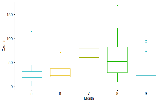
Here are five months of quality data on Ozone concentration. The task is to test if one month’s data is significantly different from any other month’s.

The first thing to graph the monthly variations of ozone in summary plots: a boxplot is one good choice.

library(ggpubr)
data("airquality")
AQ_data <- airquality
ggboxplot(AQ_data, x = "Month", y = "Ozone", 
          color = "Month", palette = c("#00AFBB", "#E7B800", "#a0AF00", "#17B800", "#20AFBB"),
        ylab = "Ozone", xlab = "Month") +
theme(legend.position="none")

Getting quantitative

Let’s do a hypothesis test. A few quick Shapiro tests suggest only month 7 followed a normal distribution. So, we will use a non-parametric test. The Kruskal–Wallis test is one of them.

kruskal.test(Ozone ~ Month, data = airquality)
	Kruskal-Wallis rank sum test

data:  Ozone by Month
Kruskal-Wallis chi-squared = 29.267, df = 4, p-value = 6.901e-06

Yes, monthly behaviours are not similar. If you want pair-wise testing, we can use a pair-wise Wilcoxon rank-sum test.

pairwise.wilcox.test(AQ_data$Ozone, AQ_data$Month)
	Pairwise comparisons using Wilcoxon rank sum test with continuity correction 

data:  AQ_data$Ozone and AQ_data$Month 

  5      6      7      8     
6 0.5775 -      -      -     
7 0.0003 0.0848 -      -     
8 0.0011 0.1295 1.0000 -     
9 0.4744 1.0000 0.0060 0.0227

P value adjustment method: holm 

The conclusion: Significant differences are seen:
Month 5 vs Month 7 and Month 8
Month 9 vs Month 7 and Month 8

Non-Parametric ANOVA – Kruskal–Wallis test Read More »

Shapiro-Wilk test – Test for Normality

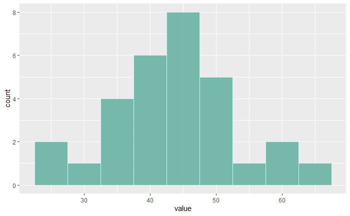
In the last post, we used a non-parametric hypothesis test, the Wilcoxon Signed Rank test. The p-value showed that the evidence was not sufficient to reject the null hypothesis. However, the histogram suggests that the data was reasonably a normal distribution.

Shapiro-Wilk test is a formal way of testing whether the data follows a normal distribution or not. The test has a null hypothesis that the sample comes from a normally distributed population. The test statistics, W has the following formula:

W = \frac{(\sum a_i x_i)^2}{\sum(x_i - \bar{x})^2}

We can apply the Shapiro-Wilk test to our data using the following R code:

diab <- c(35.5, 44.5, 39.8, 33.3, 51.4, 51.3, 30.5, 48.9, 42.1, 40.3, 46.8, 38.0, 40.1, 36.8, 39.3, 65.4, 42.6, 42.8, 59.8, 52.4, 26.2, 60.9, 45.6, 27.1, 47.3, 36.6, 55.6, 45.1, 52.2, 43.5)

shapiro.test(diab)
	Shapiro-Wilk normality test

data:  diab
W = 0.98494, p-value = 0.9361

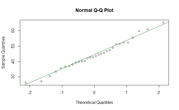
The p-value is quite high, and the null hypothesis is not rejected. The same conclusion may be obtained by doing a q-q plot as follows.

qqnorm(diab)
qqline(diab, col = "darkgreen")

Shapiro-Wilk test – Test for Normality Read More »

Wilcoxon Signed Rank Test – R Program

We will use R to perform the hypothesis test using the Wilcoxon Signed Rank Test.

The expected median age for the onset of diabetes is 45 years. The following is a list of 30 people tracking their onset of diabetes. Test whether the evidence supports the hypothesis.

diab <- c(35.5, 44.5, 39.8, 33.3, 51.4, 51.3, 30.5, 48.9, 42.1, 40.3, 46.8, 38.0, 40.1, 36.8, 39.3, 65.4, 42.6, 42.8, 59.8, 52.4, 26.2, 60.9, 45.6, 27.1, 47.3, 36.6, 55.6, 45.1, 52.2, 43.5)

The Null Hypothesis, H0: Median equals 45
The Alternate Hypothesis, H1: Median does not equal 45

wilcox.test(diab, mu = 45.0, alternative = "two.sided")
	Wilcoxon signed rank exact test

data:  diab
V = 200, p-value = 0.5158
alternative hypothesis: true location is not equal to 45

The p-value is 0.51, which is higher than 0.05 (5% significance), and therefore, the null hypothesis can not be rejected.

Since the histogram of the data appears reasonably normal, it would be interesting to test using the parametric method, such as the t-test.

t.test(diab, mu = 45.0, alternative = "two.sided")
	One Sample t-test

data:  diab
t = -0.54461, df = 29, p-value = 0.5902
alternative hypothesis: true mean is not equal to 45
95 percent confidence interval:
 40.51408 47.59925
sample estimates:
mean of x 
 44.05667 

Wilcoxon Signed Rank Test – R Program Read More »

Wilcoxon Signed Rank Test

We continue with the same dataset but use another type of non-parametric test – the Wilcoxon Signed Rank Test. Here, not only the sign of the observation counts but also the distance of departure from the median.

Case #Drug A
112.3
213.1
311.3
410.1
514.0
613.3
710.5
812.3
910.9
1011.9

The Null Hypothesis, H0: Median = 13.0
The Alternate Hypothesis, H1: Median < 13.0

Steps

  1. Estimate the difference from the null hypothesis (median = 13.0)
  2. Calculate the absolute value
  3. Estimate the rank of the list, with the smallest absolute difference getting the lowest rank
  4. Add the sign (from the difference of step 1) to the rank
  5. Add all positives and negatives separately.
  6. Take the smaller of the two and check against the table of critical values.
Drug ADifferenceAbs
Difference
RankSigned
Rank
12.3-0.70.73.5-3.5
13.10.10.111
11.3-1.71.77-7
10.1-2.92.910-10
14.01.01.055
13.30.30.322
10.5-2.52.59-9
12.3-0.70.73.5-3.5
10.9-2.12.18-8
11.9-1.11.16-6

The sum of positive ranks = 8

The sum of negative ranks = 47

We’ll take the smaller, 8 and check against the table. The number in the table (n = 10, one-sided test, alpha = 0.5) is 10. Since 8 is smaller than 10, we reject the null hypothesis.

Non-parametric tests: zedstatistics

Wilcoxon Signed Rank Test Read More »

The sign test – Continued

The sign test is a simple non-parametric test. In the last example, we went for the median of a group, classified people as + or – based on the null hypothesis and evaluated the p-value.

Here are 10 individuals undergoing a particular diet. Their haemoglobin levels are measured. Note that levels below 13.0 g/dL qualify a person as anaemic. What is your conclusion regarding the possibility of this diet inducing anaemia?

Case #Drug A
112.3
213.1
311.3
410.1
514.0
613.3
710.5
812.3
910.9
1011.9

Our task is to assess whether the group’s median haemoglobin level is 13.0 or below. Needlessly, at a specified significance level, say at 5%.
The Null Hypothesis, H0: Median = 13.0
The Alternate Hypothesis, H1: Median < 13.0

Let’s re-draw the table after including the +/- convention – plus for > 13.0 and minus for < 13.0.

Case #Drug ASign
112.3
213.1+
311.3
410.1
514.0+
613.3+
710.5
812.3
910.9
1011.9

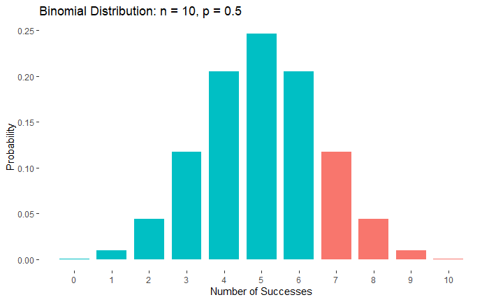
A person unexposed to statistics and random variations may conclude that at least five observations are required above 13.0 for the null hypothesis to be valid. And since there are only three, the null hypothesis is rejected. But we know about randomness and distributions, and therefore, ask this question: What is the probability of having seven negative observations from a binomial trial that is expected to have a 50% chance of success?

P(>=7) = P(7) + P(8) + P(9) + P(10) = 0.117 + 0.044 + 0.0098 + 0.001 = 0.172. In the following figure, it is the sum of the heights of the red bars.

So, the observations are unable to reject the null hypothesis. Before we end, answer this question: How many observations must be below 13.0 for the null hypothesis to be true? 

From the numbers and figure, it appears that you may need nine or ten observations below 13.0 for the sign test to make a rejection.

Does the magnitude of departure (from the median) play any role in rejecting the null hypothesis? We may have to explore another non-parametric test method, Wilcoxon signed rank, for that.

Non-parametric tests: zedstatistics

The sign test – Continued Read More »

The sign test

We have seen the definition of a non-parametric hypothesis test. The sign test is an example. We want to test the effectiveness of a drug from 12 observations. The data is the number of hours that the drug relieves pain. The null hypothesis is that the difference between paired medians equals zero.

Case #Drug ADrug B
12.03.5
23.65.7
32.62.9
42.62.4
57.39.9
63.43.3
714.916.7
86.66.0
92.33.8
1024.0
116.89.1
128.520.9

The paired differences (Drug B – Drug A) are:

data <- c(1.5, 2.1, 0.3, -0.2, 2.6, -0.1, 1.8, -0.6, 1.5, 2.0, 2.3, 12.4)

Let’s order them in the increasing magnitude.

sort(data) 
-0.6 -0.2 -0.1  0.3  1.5  1.5  1.8  2.0  2.1  2.3  2.6 12.4

Under the null hypothesis, we expect half the numbers to be above zero (median) and half below. Suppose r+ observations are > 0 and r < 0, then under the null hypothesis, r+ and r follow a binomial distribution with p = 1/2.

In our case, three cases are below zero (r), and nine are above (r+). So, we estimate the p-value in a binomial test with 9 successes out of 12, but the expected probability is 0.5 under the null hypothesis.

binom.test(9, 12,  p = 0.5, alternative = "two.sided") 
	Exact binomial test

data:  9 and 12
number of successes = 9, number of trials = 12, p-value = 0.146
alternative hypothesis: true probability of success is not equal to 0.5
95 percent confidence interval:
 0.4281415 0.9451394
sample estimates:
probability of success 
                  0.75 

Since the p-value is 0.156, we would conclude that there is no evidence of a difference between the two treatments.

The sign test Read More »