Decision Making

Hide and Seek with Camouflage

Here is another hide-and-seek game but played with an inverse handicap. If the last case would have given a clue to the seeker 75% of the time, this time, it would help the hider 75% of the time on one location, i.e., the house. So the situation is

  1. There are two options to hide – behind bushes, behind the house.
  2. If the person hides behind the house, and the opponent searches the house, there is a 75% chance the seeker will not spot the hider (camouflage effective 75% of the time.
  3. If the person hides behind the bush, and the opponent searches it, it is normal, and no camouflage works.

We have seen similar puzzles before. Suppose there was no complication of camouflage; the players should mix their choices randomly at equal probabilities (0.5).

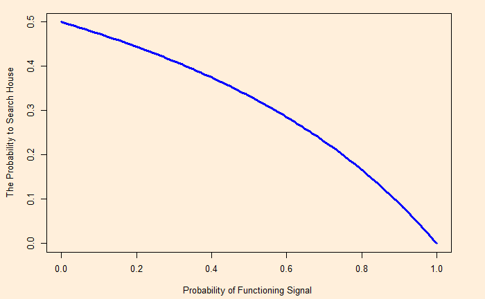
How should one search?

Let p be the probability that the seeker should search behind the house. The best value for p is such a way that the hider finds no particular incentive to choose one place over the other. In other words, the p makes the payoffs for the hider to hide behind bush and house equal.

Payoff to hide behind house = Payoff to hide behind bushes.
Pay off for hide behind house = p[1 x 0.75 + 0 x 0.25] + (1-p) x 1 = 0.75p + 1 – p
Pay off for hiding behind bushes = p x 1 + (1-p) x 0 = p

If the hider hides behind the house and the seeker searches the house, there is a 75% probability that she will gain one point and a 25% chance of zero. On the other hand, if the hider is behind the house and the seeker searches the bush, the hider gets a full score (one).

Solving for p,
0.75p + 1 – p = p
p = 0.8

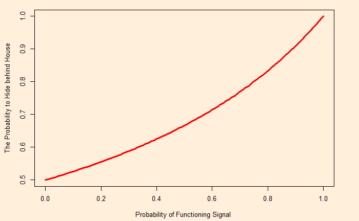
How should one hide?

Let q be the probability that the hider must hide behind the house. Following the logic as before,

Payoff to search behind house = Payoff to search behind bushes.
Payoff to search behind house = q[0 x 0.75 + 1 x 0.25] + (1-q) x 0 = 0.25q
Payoff to search behind bushes = q x 0 + (1-q) x 1 = 1 – q

Solving for q,
0.25q = 1 – q
q = 0.8

Reference

Camouflaged Hide and Seek: William Spaniel

Hide and Seek with Camouflage Read More »

Hide and Seek Continued

We have seen a counterintuitive solution to the particular hide-and-seek game in which a signal (light) comes up at a fixed probability from one of the locations should one choose to hide there. Here is how one should hide, given the chance of the signal from the very location.

Let’s develop some intuition over the message from the plot. When there is no signal from one of the locations (the house), it becomes a normal hide-and-seek, and the person who hides must choose both places randomly at a 50:50 chance. On the other hand, when there is a signal from the house, the seeker can use it to her advantage, as some of the uncertainty over hiding behind the house gets eliminated by the presence of a signal and can search the other place more often. Once you understand the seeker’s mind, the hider must choose the house more often to counter the opponent.

The extreme case is when the probability of the signal is 99.99%, where the seeker can almost ignore the house and concentrate on the bushes. And that’s what the seeker will do, as seen in the plot below.

Hide and Seek Continued Read More »

Hide and Seek of the Second Order

Annie and Becky are playing hide and seek. Annie wants to hide, and it’s Becky’s job to find out. Annie has two choices – hide behind a house or the bushes. But there is a problem: if she hides behind the hose, there is a 75% probability that the surveillance system will catch her and a light will lit in the front. How often should Annie try to hide behind the house?

We have seen similar puzzles before. Suppose there was no complication due to light. In that case, intuition suggests that Annie and Becky should mix their choices randomly at equal probabilities.

Probabilities for searching

Becky’s strategy is designed to make both choices equally attractive to Annie. Let p be the probability that Becky search the house. Then, for Annie, the payoffs much match.

Hide behind house = Hide behind bushes.
Pay off for hide behind house = 0 x 0.75 + 0.25 [0 x p + 1 x (1-p)].
Pay off for hiding behind bushes = 1 x p + 0 x (1-p)

Explanation for the first equation. If Annie hides behind the house, there is a 75% probability that the light will lit and Becky will go and find her (or Annie ends up with 0). On the other hand, inside the 25% case, where no light is lit, there is a p chance Becky will go for the house and a (1-p) chance Becky will miss.

Solving for p,
0.25 – 0.25 p = p
p = 0.2

Probabilities for hiding

Let q be the probability for Annie to hide behind the house. Note that Becky will need to apply probabilities only when there is no light in front of the house. Annie’s strategy is to make payoffs for Becky equal (given no light).

The chance that Annie hides behind the house given no light is a conditional probability, and we must apply Bayes’ rule.

P(HH|NL) = P(NL|HH) x P(HH) / [ P(NL|HH) x P(HH) + P(NL|HB) x P(HB)]
= 0.25q /[0.25q + (1-q)]

Similarly, The probability Annie hides behind the bushes given no light is:
P(HB|NL) = P(NL|HB) x P(HB) / [P(NL|HB) x P(HB) + P(NL|HH) x P(HH)]
= (1-q) /[(1-q) + 0.25q]

Now, back to payoffs:

Payoff for Search house | no light = Payoff for Seach bushes | no light
Payoff for Search house | no light = 1 x [0.25q /[0.25q + (1-q)]] + 0 x (1-q) /[(1-q) + 0.25q]
Payoff for Search bushes | no light = 0 x [0.25q /[0.25q + (1-q)]] + 1 x (1-q) /[(1-q) + 0.25q]

0.25 q /[0.25q + (1-q)]] = (1-q) /[(1-q) + 0.25q]
0.25 q = (1-q)
q = 1/1.25 = 0.8

This is counterintuitive; Annie will hide behind the house 80% of the time, knowing the light will be lit 75% of those occasions.

Reference

Expert-Level Hide and Seek: William Spaniel

Hide and Seek of the Second Order Read More »

Banzhaf Power Index – Continued

The calculation of the Banzhaf Power Index is as follows.

  1. List all winning coalitions
  2. In each collision, identify the critical players
  3. Count how many times each player is critical
  4. Convert these counts to fractions by dividing them by how many times any player is critical.

Here are a few definitions before we go further:

  1. A coalition is a group of players voting the same way
  2. Winning coalition: If the total weight of the coalition is equal to or greater than the quota, it is a winning coalition.
  3. Critical player: If by leaving the coalition, a player in a coalition makes a winning coalition into a losing one.

All coalitions

Following are all the three-player combinations

PP <- c(15, 25, 10, 30, 20)

PP_Comb <- combinations(n = 5, r = 3, v = PP, set = FALSE)
P2_Comb <- as.data.frame(PP_Comb) 
P2_Comb$Sum <- rowSums(PP_Comb) 
PlayerPlayerPlayerTotal WeightWinning
Coalition
15251050NO
15253070YES
15252060YES
15103055YES
15102045NO
15302065YES
25103065YES
25102055YES
25302075YES
10302060YES

All four-player combinations

PP <- c(15, 25, 10, 30, 20)

PP_Comb <- combinations(n = 5, r = 4, v = PP, set = FALSE)
P2_Comb <- as.data.frame(PP_Comb) 
P2_Comb$Sum <- rowSums(PP_Comb) 
PlayerPlayerPlayerPlayerTotal WeightWinning
Coalition
1525103080YES
1525102070YES
1525302090YES
1510302075YES
2510302085YES

Finally, the 5-player combination: 15, 25, 10, 30, 20 = 100

The table of all the winning coalitions with critical players in bold follows.

P2,P4 (25,30)
P1, P2, P4 (15, 25, 30)
P1, P2, P5 (15, 25, 20)
P1, P3, P4 (15, 10, 30)
P1, P4, P5 (15, 30, 20)
P2, P3, P4 (25, 10, 30)
P2, P3, P5 (25, 10, 20)
P2, P4, P5 (25, 30, 20)
P3, P4, P5 (10, 30, 20)
P1, P2, P3, P4 (15, 25, 10, 30)
P1, P2, P3, P5 (15, 25, 10, 20)
P1, P2, P4, P5 (15, 25, 30, 20)
P1, P3, P4, P5 (15, 10, 30, 20)
P2, P3, P4, P5 (25, 10, 30, 20)
P1, P2, P3, P4, P5 (15, 25, 10, 30, 20)
PlayerCritical
Times
Banzhaf
Power Index
P133/26
=11.5%
P277/26
= 26.9%
P322/26
= 7.7%
P499/26
= 42.3%
P555/26
= 19.2%
Total26

Player 4 has the highest voting power, with Banzhaf Power Index = 42.3%.

Banzhaf Power Index – Continued Read More »

Banzhaf Power Index

Let’s continue from the previous voting weights of five shareholders. This time, we calculate the power in the weighted voting system and determine the critical players. We use R functions to simplify the work. But first, the voting system:
[51: 15, 25, 10, 30, 20]
The shorthand notation indicates that 51% is required to reach the quota, and the players 1 to 5 have 15%, 25%, 10%, 30%, and 20% voting weights, respectively.

The calculation of the Banzhaf Power Index is as follows.

  1. List all winning coalitions
  2. In each collision, identify the critical players
  3. Count how many times each player is critical
  4. Convert these counts to fractions by dividing them by how many times any player is critical.

All coalitions

Following are all the two-player combinations

combinations(n = 5, r = 2, v = c("P1", "P2", "P3", "P4", "P5"))
      [,1] [,2]
 [1,] "P1" "P2"
 [2,] "P1" "P3"
 [3,] "P1" "P4"
 [4,] "P1" "P5"
 [5,] "P2" "P3"
 [6,] "P2" "P4"
 [7,] "P2" "P5"
 [8,] "P3" "P4"
 [9,] "P3" "P5"
[10,] "P4" "P5"

And their weights,

PP <- c(15, 25, 10, 30, 20)
PP_Comb <- combinations(n = 5, r = 2, v = PP, set = FALSE)
P2_Comb <- as.data.frame(PP_Comb) 
P2_Comb$Sum <- rowSums(PP_Comb) 
PlayerPlayerTotal WeightWinning
Coalition
152540NO
151025NO
153045NO
152035NO
251035NO
253055NO
252045NO
103040NO
102030NO
302050NO

We’ll continue with the other player combinations in the next post.

Banzhaf Power Index Read More »

Weighted Voting

Weighted voting is a concept in which voters with different numbers of votes or influences determine the outcome of an election. The more votes someone holds, the more weight she gets in deciding the result. A simple example is a shareholder meeting where 51% of votes are required to settle a decision. Five shareholders hold 15%, 25%, 10%, 30%, and 20% of the total shares. Each of the shareholders gets a weightage corresponding to the shares they hold.

A: 15%
B: 25%
C: 10%
D: 30%
E: 20%
In the above example, Player D gets the highest weight, and Player C has the lowest. Quota is the minimum weight required to pass the election. And in our case, the quota is 51%.

If q represents the quota, w1, w2, etc., denotes the weight of player 1, player 2, etc., then the shorthand notation of the voting system is written as:
[q: w1, w2, w3, w4, w5]

In our example, it is
[51: 15, 25, 10, 30, 20]

Dictator: When one entity has a weight equal to or more than the quota. There is no dictator in [51: 15, 25, 10, 30, 20], but the third entity is a dictator in [51: 10, 20, 52, 18]. A dictator can pass or block any resolution, and nobody can win a vote without the dictator.

A player has veto power if her support is necessary to reach the quota. In [10: 6, 5, 4], player 2 and player 3 can only get the quota with support from player 1. Player 1 has veto power. On the other hand, player 2 or player 3 has no veto power. No one has veto power in [10, 6, 5, 7].

A player is a dummy if her vote is never essential for a group to reach quota. Player 3 is a dummy in [10: 7, 4, 2].

Weighted Voting Read More »

Airport Problem and the Shapley Solution

Here is how we apply the concept of Shapley Values to the famous airport problem.
Suppose an airport wants to build a runway to support three airline companies. Here are the requirements for each company:
Airline 1: 1500 m
Airline 2: 2200 m
Airline 3: 3000 m
Assume the cost per m of runway construction is $1k. How must the airport split costs among the three airline companies fairly?

Proportional rule

The simplest way is to split the cost proportional to the length each airliner needs, i.e., you divide the total cost proportional to the runway requirements as:

Airline 1: 3000 x 1500 / (1500 + 2200 + 3000 ) = 672k
Airline 2: 3000 x 2200 / (1500 + 2200 + 3000 ) = 985k
Airline 3: 3000 x 3000 / (1500 + 2200 + 3000 ) = 1343k

Is it a fair division? It seems so. But what happens if Airline 3 comes up with a variation, say, change to 3500? The new contributions get modified to:
Airline 1: 729k
Airline 2: 1069k
Airline 3: 1701k

Suddenly, this seems unfair for Airlines 1 and 2 as the new plan only benefits the third one, but the others also bear the extra costs (729 – 672) and (1069 – 985), respectively. So, we try the Shapley values:

Shapley value

We have seen how it works in the previous post. Let’s build the table first for case 1.

C(1500, 2200, 3000)

Combination 123
1231500700800
132150001500
23102200800
21302200800
312003000
321003000
Average3000/6
= 500
5100/6
= 850
9900/6
= 1650

And for case 2, C(1500, 2200, 3500):

Combination 123
12315007001300
132150002000
231022001300
213022001300
312003500
321003500
Average3000/6
= 500
5100/6
= 850
12900/6
= 2150

Case 1:
Shapley value Airline 1 = 500
Shapley value Airline 2 = 850
Shapley value Airline 3 = 1650

Case 2:
Shapley value Airline 1 = 500
Shapley value Airline 2 = 850
Shapley value Airline 3 = 2150

The game theory solution does not penalise the first two airlines and only demands the third one to pay for the scope change.

Airport Problem and the Shapley Solution Read More »

Shapley Value

Three people – Andy, Bichel and Carol decided to share a taxi to reach their homes. Andy will get down first, where the taxi fare if travelled alone, would have been $5; Bichel should have paid $10 and Carol 25. How should they divide the taxi fair?

It does not make sense, Andy – $5, Bichel $10 and Carol $25 as it would mean paying $40 for the taxi!
It’s not fair on Andy if he is asked to pay 5, Bichel 5 (10-5, marginal fare) and Carol 15 (25 -10).

Lloyd Shapley introduced a concept known as the Shapley Value, based on the notion of fairness to divide the payoff among all the coalition members.

The Shapley value is the average of marginal contributions of all the permutations of the three individuals. First, how many permutations are possible? It is 3! or 6.

ABC
ACB
BCA
BAC
CAB
CBA

The marginal contribution is calculated assuming A, B, and C came to the coalition in that order. ABC implies A comes first and pays 5, B comes then and pays his fare minus (-) what is already paid (10-5), and C pays 25 – 10. In the same way, CAB means C pays 25, A pays 0, and B pays 0. Let’s tabulate the marginal contributions.

Combination ABC
ABC5515
ACB5020
BCA01015
BAC01015
CAB0025
CBA0025
Average10/6
= 1.67
25/6
= 4.17
115/6
19.17

The Shapley value of Andy is $1.67
The Shapley value of Bichel is $4.17
The Shapley value of Carol is $19.17
If you add all the contributions up, you get $25.

Shapley Value Read More »

Causal Diagrams

A causal diagram is a graphical representation of the relationship between variables. For example, the picture below describes a probability rule specifying how Y changes if X changes.

Back-door path

Is any path from X to Y that starts with an arrow pointing to X. Here is an example with a back-door path (X <- Z -> Y)

Whereas the picture below has no back-door path

Confounder

We know what a confounder is, and it is an example of a back-door path. The most famous example is the relationship between sunburn and ice cream sales! The data may show sunburn increases with ice cream sales. In contrast, the proper interpretation requires a back-door path in which a confounder, sunlight, causes both an increase in ice cream sales and sunburn.

Mediator

An example of a mediator is the case of an alarm for fire hazards. Here, smoke is a mediator; when a fire happens, the detector detects the smoke and sets off the alarm.

Causal Diagrams Read More »

Three Cards

A bag contains three cards – one is red on both sides, the second is white on both sides, and the third is red on one side and white on the other. Amy draws a card without looking and keeps it on the table. If the card is red face up, what is the probability that it’s also red on this hidden side?

Intuition tells the probability to be 1/2. The argument goes like this: if the side up is red, there are two equal possibilities for the hidden side – red or white. Therefore, it’s 1/2. A slightly different version of the same logic estimates that once the person sees it red, it shuts the options white-white card, leaving only two red-red and red-white. The card must be one out of two.

Conditional Probability

Let’s investigate the problem using conditional probability (the Bayes’ rule).

P(RR|Ru) represents the required probability, or the card is RR given R is up.

P(RR|R_u) = \frac{P(R_u|RR)P(RR)}{P(R_u|RR)P(RR) + P(R_u|RW)P(RW)}

P(Ru|RR) = probability of red up given RR is the selected card
P(RR) = Prior probability of choosing the RR card
P(Ru|RW) = probability of red up given RW is the picked card
P(RW) = Prior probability of selecting the RW card

P(Ru|RR) must be 1 as RR will always show red up
P(RR) = 1/3, as there are three cards to choose from
P(Ru|RW) = 1/2, there is a 50:50 chance for red to show up from an RW card
P(RW) = 1/3

P(RR|R_u)= \frac{1 * 1/3}{1 * 1/3 + 1/2 * 1/3} = \frac{2}{3}

Three Cards Read More »