Decision Making

Logistic Regression and R

We have seen logistic regression as a means to estimate the probability of outcomes in classification problems where the response variable has two or more values. We use the ‘Default’ dataset from ‘ISLR2’ to illustrate. The data set contains 10000 observations on the following four variables:

default
: A factor with levels No and Yes indicating whether the customer defaulted on their debt

student:
 factor with levels No and Yes indicating whether the customer is a student

balance: 
The average balance that the customer has remaining on their credit card after making their monthly payment
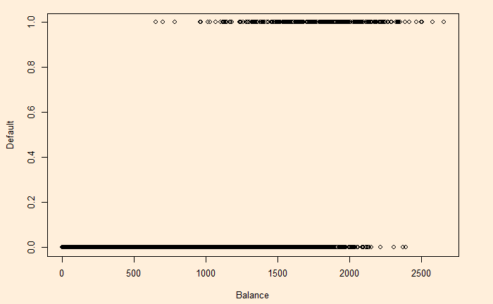
income: Income of customer

We change YES to 1 and NO to 0 and plot default vs balance.

Let p(X) be the probability that Y = 1 given X. The simple form that fits this behaviour is:

P(X) = \frac{e^{\beta_0 + \beta_1 X}}{1 + e^{\beta_0 + \beta_1 X}}

The beta values (the intercept and slope) are obtained by the ‘generalised linear model’, glm function in R.

D_Data <- Default
D_Data$def <- ifelse(D_Data$default=="Yes",1,0)
model <- glm(def ~ balance, family = binomial(link = "logit"), data = D_Data)
summary(model)

Call:
glm(formula = def ~ balance, family = binomial(link = "logit"), 
    data = D_Data)

Deviance Residuals: 
    Min       1Q   Median       3Q      Max  
-2.2697  -0.1465  -0.0589  -0.0221   3.7589  

Coefficients:
              Estimate Std. Error z value Pr(>|z|)    
(Intercept) -1.065e+01  3.612e-01  -29.49   <2e-16 ***
balance      5.499e-03  2.204e-04   24.95   <2e-16 ***
---
Signif. codes:  0 ‘***’ 0.001 ‘**’ 0.01 ‘*’ 0.05 ‘.’ 0.1 ‘ ’ 1

(Dispersion parameter for binomial family taken to be 1)

    Null deviance: 2920.6  on 9999  degrees of freedom
Residual deviance: 1596.5  on 9998  degrees of freedom
AIC: 1600.5

Number of Fisher Scoring iterations: 8

Now, we will test how good the model predictions are by plotting the function using the regressed beta0 ( = -10.65) and beta1 (= 0.0055).

plot(D_Data$balance, D_Data$def, xlab = "Balance", ylab = "Default")

y <- function(x){
  exp(-10.65+0.0055*x) / (1 + exp(-10.65+0.0055*x))
}

x <- seq(0, 3000)
lines(x, y(x), col = "red")

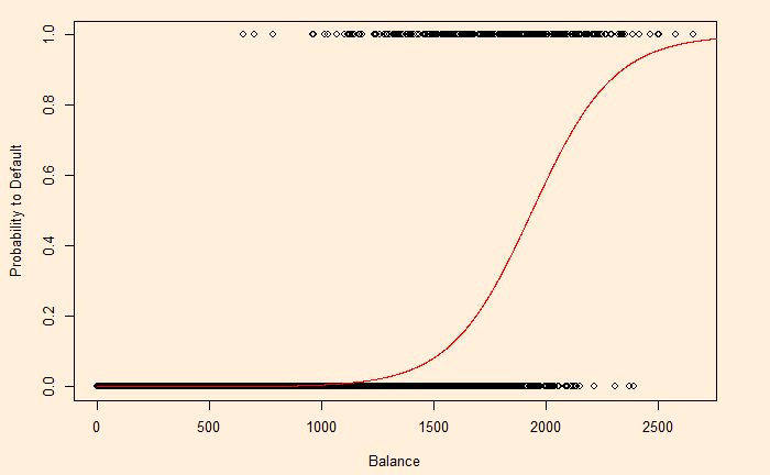
But R has an even simpler way to get this curve.

plot(D_Data$balance, model$fitted.values)

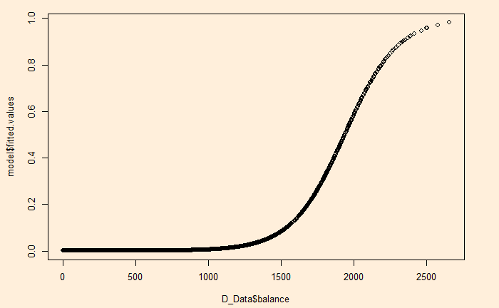
Logistic Regression and R Read More »

Borda count Method

Border Count is another method to determine the winner of a voting scheme. As per Wiki, the technique was first proposed in 1435 by Nicholas of Cusa but is named after the French mathematician Jean-Charles de Borda, who developed the system in 1770.

In this method, points are given to candidates based on their ranking:

  1. The last one gets 1 point
  2. The second-to-last gets 2 points, and so on.
  3. The points are totalled, and the one who gets the maximum points is the winner.

Here is our previous example:

# Voters412513263015
1st ChoiceLLFFCC
2nd ChoiceFCLCFL
3rd ChoiceCFCLLF

Points are given as follows:
First place: 3 points
Second Place: 2 points
Third place: 1 point

# Voters412513263015
1st Choice
(3 pts)
L
41×3
123
L
25×3
75
F
13×3
39
F
26×3
78
C
30×3
90
C
15×3
45
2nd Choice
(2 pts)
F
41×2
82
C
25×2
50
L
13×2
26
C
26×2
52
F
30×2
60
L
15×2
30
3rd Choice
(1 pt)
C
41×1
41
F
25×1
25
C
13×1
13
L
26×1
26
L
30×1
30
F
15×1
15

L: 123 + 75 + 26 + 30 + 26 + 30 = 310 points
F: 39 + 78 + 82 + 60 + 25 + 15 = 299 points
C: 90 + 45 + 50 + 52 + 41 + 13 = 291 points

Under the Borda count method, L is the winner.

Borda count Method Read More »

Charlie Munger’s Wisdom – Continued

We saw the first 10 of the 24 Cognitive Biases from Charlie Munger’s 1995 speech – Human Misjudgement. In this post, we will go through the rest.

11. Bias from deprival super-reaction syndrome: This is akin to the loss aversion bias, illustrating how we react when possessions, even trivial ones, are taken away. Consider, for instance, the intensity of employee-management negotiations where every inch is fiercely contested.

12. Bias from envy/jealousy:

13. Bias from chemical dependency, 14. Bias from gambling dependency: These biases don’t need a lot of explanation. They trigger attentional bias, leading individuals to allocate disproportionally more attention to addiction-relevant cues than to neutral stimuli. Businesses, whether pubs or casinos, are well-versed in exploiting these vulnerabilities. Being aware of these tactics can help you navigate such situations more effectively.

15. Bias from liking distortion: It’s about liking oneself, one’s ideas, and community. And making stupid ideas only because they came from someone you liked.

16. Bias from disliking distortion: Opposite of liking distortion. In this case, you dismiss ideas from people who you don’t like.

17. Bias from the non-mathematical nature of the human brain: Human brains in their natural state (i.e., untrained state) are notoriously inefficient when dealing with probabilities. Within this entity, Munger conveniently folds various fallacies of the human mind – crude heuristics, availability, base-rate neglect, hindsight – into one.

18. Bias from fear of scarcity: The fear of scarcity can bring out pure dumbness in otherwise perfectly normal people. A familiar example is the toilet paper rush during the early days of the Covid pandemic.

19. Bias from sympathy: It’s about leaders keeping employees with dubious personal qualities. Often, this happens out of pity for the person or her family. Munger says that while paying them the proper severance is essential, keeping such people in jobs can make the whole organisation poor.

20. Bias from over-influence and extra evidence:

21. Bias caused by confusion due to information not being properly processed by the mind: Munger stresses the need to understand the reasons (answer to the question – why?) for the information to be properly registered in the brain. Like for individuals themselves, it is also important for people to explain the reasoning clearly while communicating the key decisions and proposals to their stakeholders.

22. Stress-induced mental changes: What later happened to the Pavlovian dogs (conditioned for certain behaviours) after their cages were flooded was a good example of what stress can do. The canines forgot all the training and responses that they had acquired.

23. Common mental declines:

24. Say-something syndrome: It’s a habit of many individuals to do the talk irrespective of their expertise and capacities to impact the decision-making process. They remain just soundbites, and Munger cautions to watch out for those quiet selves that eventually add quality.

Charlie Munger’s Wisdom – Continued Read More »

Charlie Munger’s Wisdom

One of the greatest investors in history, Charles Munger, passed away on the 28th of November 2023, 33 days short of his 100th birthday. His celebrated talk at Harvard University in 1995 on the subject of ‘Human Misjudgment’ is undoubtedly a masterclass about the patterns of human irrationality. This and the next posts are about those 24 tendencies of the human brain that Mr Munger has immortalised in his celebrated lecture.

1. Underrecognition of the power of incentives: Munger illustrates his point using the cases of FedEx and Xerox, demonstrating that it was not logic but incentives that drove their employees. The incentives were intended to speed up work and improve sales. However, the workers maximised the commissions and overtime by selling inferior products and working longer.

2. Psychological denial: It is a type of mechanism by the brain to avoid reality, as it can cause deep pain and anxiety. Examples are parents refusing to believe the loss of their children or youths getting into crimes.

3. Incentive-caused bias: It’s also known as the Principal-Agent problem in companies. The people entrusted to lead companies (on behalf of the owners/shareholders) erode the long-term value of companies (principals’ interest) by going after short-term fixes or management’s vested interests (agent’s gain).

4. Self-confirmation bias: People tend to persist on already-made conclusions even when (newly) available evidence disproves them.

5. Bias from cognitive dissonance: It is similar to the earlier one. Cognitive dissonance bias is the mental discomfort that a person goes through if they have to hold two conflicting views about something. Most often, the receiver of the new information revolts with it, leading to selective perception and decision-making.

6. Bias from Pavlovian association: This refers to the famous experiments on dogs carried out by Pavlov. The experiments prove a great deal about the mental shortcuts of humans in making decisions. In other words, people choose a ‘go’ for an incentive stimulus, whereas they select a ‘no go’ on punishment stimuli. A wonderful example is how advertisements work in our minds.

7. Bias from reciprocation tendency: Humans return favour when they receive something from others. While this may seem a virtue, the behaviour can be manipulated, compelling individuals to substantially lower the cost of services.

8. Bias from over-influence of social proof: This is the absolute compliance to the ‘wisdom of the crowd’ or inability to act against social norms. Social proof works in unclear social situations where people follow what the surrounding people do. Munger gives an example of how all major oil companies started buying fertiliser companies when one of them initiated the trend. Another term closely related to this topic is the ‘power of reinforcement‘. Typical causes of bull or bear runs of stock markets.

9. Bias from distortions caused by distortion, sensation, and perceptions: In Cialdini’s famous experiment, students who first dipped their hands in hot water felt cold and cold water felt hot on a subsequent dip in the water at room temperature. He cites the familiar trick of a real estate broker who manages to sell her client a moderately over-priced house by first showing an outrageously overpriced house.

10. Bias from over-influence by authority: It is a tendency of the brain to be influenced by the opinion of an authority figure, even when the content is inaccurate. Like all cognitive biases, the authority bias is a shortcut our brains use to save energy in decision-making.

Reference

The Psychology of Human Misjudgement – Charlie Munger Full Speech: Warren Buffett

Charlie Munger’s Wisdom Read More »

Voting Theory: Instant Runoff

Instant run-off voting, also called the plurality with elimination, is a modification of the plurality method. This method removes the candidate with the least first-place votes, and the votes for the now-eliminated candidate are redistributed to the voter groups’ next choice. It continues until a candidate gets the majority (> 50%).

# Voters412513263015
1st ChoiceLLFFCC
2nd ChoiceFCLCFL
3rd ChoiceCFCLLF

Look at the previous example: L (for library) wins after getting 66 out of the possible 150 votes. For a majority, a candidate must get 76 votes.
L: 66
F: 39
C: 45
IRV method eliminated the last one, F. The table now looks like the following.

# Voters412513263015
1st ChoiceLLCC
2nd ChoiceCLCL
3rd ChoiceCCLL

The two empty entries against the 1st choice now go to the ones below – 13 to L and 26 to C. The updated votes are:
L: 79
C: 71

L now becomes the winner of the Instant run-off voting method.

Voting Theory: Instant Runoff Read More »

Condorcet Criterion

In the earlier post, we saw how the plurality method of voting works. In the plurality method, the choice with the most first preference votes is declared the winner. In the example, the library won the election event (with 66 out of 150 first-choice votes), although it did not get a majority.

# Voters412513263015
1st ChoiceLLFFCC
2nd ChoiceFC LCFL
3rd ChoiceCFCLLF

Condorcet criterion

If there is a winner in this case that wins every one-to-one comparison, we call it a Condorcet winner. Let’s find out who the Condorcet winner is in the earlier example.

Step 1: Ignore the one not in the comparison
Step 2: Add all votes of each
Step 3: The one that has the most votes is the winner of the matchup

L vs F

# Voters412513263015
1st ChoiceLLFF
2nd ChoiceFLFL
3rd ChoiceFLLF

L is preferred over F by 41 + 25 + 15 = 81 votes
F is preferred over L by 13 + 26 + 30 = 69 votes
L wins the matchup

C vs F

# Voters412513263015
1st ChoiceFFCC
2nd ChoiceFC CF
3rd ChoiceCFCF

C = 25 + 30 + 15 = 70
F = 41 + 13 + 26 = 80
F wins

L vs C

# Voters412513263015
1st ChoiceLLCC
2nd ChoiceC LCL
3rd ChoiceCCLL

L = 41 + 25 + 13 = 79
C = 26 + 30 + 15 = 71
L wins

Since L wins both its one-to-one comparisons, it becomes the Condorcet winner.

Condorcet Criterion Read More »

Voting Theory: Plurality Method

In the plurality method, the choice with the most first preference votes is declared the winner. It is possible to have a winner in the plurality method without having a majority over 50%. Here is an example of a preference table:

Six voting blocks made their preferences for a city project. The options are to build a Library (L), Fitness Centre (F) or a commercial complex (C).

# Voters412513263015
1st ChoiceLLFFCC
2nd ChoiceFCLCFL
3rd ChoiceCFCLLF

Here are the aggregates of first-choice votes for each option.

ChoiceVotes%
Library(L)6666/150
= 44
Fitness (F)3929/150
= 26
commercial (C)4545/150
= 30

The library is the winner.

The plurality method can potentially violate fairness criteria as the final choice is not guaranteed to win in all one-to-one comparisons. One of them is the Condorcet Criterion.

Voting Theory: Plurality Method Read More »

Braess’s Paradox

Another counterintuitive experience similar to Downs–Thomson’s is Braess’s Paradox. As per this phenomenon, adding more roads to an existing network can slow down the overall traffic. Similar to the previous, we will see the mathematical explanation first.

Suppose there are two routes to city B from city A, as shown in the picture – the top and bottom roads. The first part is narrow on the top road, followed by a broad highway. The situation is the opposite for the bottom road.

The highways are not impacted by the number of cars, whereas, for the narrower roads, the traffic time is related to the number of vehicles on the road – N/100, where N is the number of cars.

If there are 1000 cars in the city, the system will reach the Nash equilibrium by cars getting equally divided (in the longer term), i.e., 500 on each road. Therefore, each car to take
500/100 + 15 = 20 mins

Imagine a new interconnection built by the city to reduce traffic congestion. The travel time on the connection section is 1 minute. Let’s look at all scenarios.

Scenario 1: A car starts from the bottom highway, takes the connection, and moves to the top highway. Total time = 15 + 1 + 15 = 31 mins.
Scenario 2: One car starts from the top road, takes the connection, and moves to the bottom road, while the others follow the old path (not using the connection). Total time = 50/100 + 1 + 51/100 ~ 11 mins.

Scenario 2 seems a no-brainer to the car driver. But this news invariably reaches everyone, and soon, everyone starts taking the narrow paths! In other words, the narrow route is the dominant strategy. The total travel time now becomes:
1000/100 + 1 + 1000/100 = 21 min. This is more than the old state, a situation with no connection possible.

So, the condition without the connection road (or closing down the connection road) seems a better choice. And this is Braess’s paradox suggesting that a more complex system may not necessarily be a better choice.

Braess’s Paradox Read More »

Downs–Thomson paradox

Here is a game theory puzzle for you. The government proposes to build a highway between the two cities, A and B, that reduces the burden of the existing freeway. Here is the rationale behind the proposal.

There are two modes of arriving from A to B: 1) take the train, which takes 20 minutes, or 2) take the freeway using a car, which takes (10 + n/5) minutes, where n is the total number of cars on the road. Since the train is a public transit, it doesn’t matter how many people take it – it always takes 20 minutes to reach the destination. But if the new highway operates, the travel time becomes (5 + n/5) minutes. Note that the old freeway stops functioning once the new road is available.

What is your view on building the highway as a solution to reduce travel time, or are there alternate ideas to meet the objective?

The existing case

Suppose there are 100 commuters. Each can take the train and reach B in 20 minutes. That gives a few people the advantage of taking cars and reaching their destination earlier – until the travel time matches the following way.
20 = 10 + n/5
n = 50
Beyond 50 commuters, car travel will take longer than the train; therefore, 50 is an equilibrium number in the longer term.

The new case

The new equilibrium is estimated as follows:
20 = 5 + n/5
n = 75
In other words, more people will take the new route, but the travel time remains the same.

The paradox

This is a simplified game-theory explanation of what is known as the Downs–Thomson paradox. It says that comparable public transport journeys or the next best alternative defines the equilibrium speed of car traffic on the road.

Alternatives

On the other hand, if modifications are possible to reduce the commute time of the train, then overall travel time (for both railways and roads) can be reduced.

References

Downs–Thomson paradox: Wiki

The Problem with Faster Highways: William Spaniel

Downs–Thomson paradox Read More »

The Auction Game

Amy and Becky are in an auction for a painting. The rules of the auction are:

  1. Bidders must submit one secret bid.
  2. The minimum amount to bid is $10 and can be done in increments of $10
  3. Whoever bids the highest wins and will be charged an amount equal to the bid amount.
  4. In the event of a tie, the auction house will choose a winner based on a lot with equal probabilities.

Amy thinks the fair value of the painting is $56, and Becky thinks it’s $52. These valuations are also known to both. What should be the optimal bid?

The payoff matrix is:

Becky
Bid $40Bid $50
AmyBid $408, 60, 2
Bid $506, 03, 1

If Amy bids $40 and Becky $50, Becky wins the painting and her payoff is the value she attributes (52) – the payment (50)= $2. The loser wins or loses nothing.
If Amy bids $50 and Becky $40, Amy gets it, and her payoff will be the value (56) – what she pays (50) = $6.
If both bid at $40, Amy can get a net gain of 16 (56 – 40) at a probability of 0.5. That implies the payoff for Amy = $8. For Becky, it’s $12 x 0.5 = $6.
If both bid for $50, Amy’s payoff = $6 x 0.5 = $3 and Becky’s = $2 x 0.5 = $1

At first glance, it seems obvious that the equilibrium is where both are bidding for $40. If Amy thinks Becky will bid $40, Amy’s best response is to bid the same as her payoff is $8. The same is the case for Becky.
But if Amy expects Becky to go for $50, then Amy must also bid $50. Becky will also go along the same logic.

The Auction Game Read More »