Data & Statistics

What’s Wrong With Coffee?

Conflicting reports on the health benefits of drinking coffee is a topic of debate and confusion, often made science and scientists subjects of jokes. Over the years, several researchers have tried to establish associations between consuming coffee and a bunch of outcomes such as hypertension, cancer, gastrointestinal diseases – you name it.

Why these discrepancies?

Many of these studies are observational and not interventional. To make the distinction, cohort studies are observational, whereas randomised controlled trials (RCTs) are interventional. Establishing causations from observational studies is problematic.

In addition, coffee contains over 2000 active components, and theorising their impact on physiology, with all possible synergistic and antagonistic effects, is next to impossible. See these observations: taking caffeine as a tablet causes four times the elevation of blood pressure compared to drinking caffeinated coffee. There is an association of elevated BP with caffeinated drinks but none with coffee. So, accept this is complex.

Jumping to a conclusion is another issue. Researchers are often under tremendous pressure to publish. And like journalists, they too get carried away by results with sensation content. As a result, the authors (and readers) advertise relative risks as absolute risks, forget confidence intervals, shun the law of large numbers (or the absence of the law of small numbers) or ignore confounding factors!

Confounders

How will you respond when you hear a study in the UK that found an association between coffee drinking and elevated BP? First, who are those coffee drinkers in the land traditionally of tea lovers? If it was the cosmopolitan crowd, are there lifestyle factors that can have a confounding effect on the outcome of the study: working late hours, lack of exercise, higher stress levels, skipping regular meals, smoking?

The same goes for the beneficial effect of coffee on Parkinson’s disease. What if I argue that people with a tendency to develop the disease are less interested in developing such addictions due to the presence or absence of certain life chemicals? In that case, it is not the coffee that reduced Parkinson’s, but a third factor that controlled both.

Absolute or Relative

The risk of lymphoma is 1.29 for coffee drinkers, with a confidence interval ranging from 0.92 to 1.8. What does that mean? 30% of people who drink coffee get lymphoma? Or a relative risk with a wide enough interval that enclosed one inside it? If it is a relative risk, what is the baseline incident rate of lymphoma? More questions than answers.

Meta-analysis

Meta-analysis is a statistical technique that combines data from several already published studies to derive meaning. A meta-analysis, if done correctly, can bring the big picture from the multitudes of individual findings. The BMJ publication in 2017 is one such effort. They collected more than 140 articles published on coffee and its associated effects that provided them with more than 200 meta-analyses, including results from a few randomised controlled studies.

The outcome of the study

  1. Overall, coffee consumption seems to suggest more benefits than harm!
  2. 4% (relative risk)[0.85-0.96] reduction in all-cause mortality.
  3. A relative risk reduction of 19% [0.72-0.90] for cardiovascular diseases.
  4. Same story for several types of cancers, except for lung cancer. But then, the association of a higher tendency for lung cancer was reduced when adjusted for smoking. For non-smokers, on the other hand, there is a bit of benefit, like in the case of other cancers.
  5. Consumption of coffee leads to lower risks for liver and gastrointestinal outcomes—similar association for renal, metabolic, and neurological diseases such as Parkinson’s.
  6. Finally, something bad: harmful associations are seen for pregnancy, including low birth weight, pregnancy loss, and preterm birth.
  7. Many of these associations are marginal, and also the domination of observational data reduces the overall quality of conclusions. These results would benefit from more randomised controlled trials before formalising.

Meta-Analysis: NCBI

Randomised Controlled Trials: BMJ

Confounders contributing to the reported associations of coffee or caffeine with disease: NCBI

Coffee consumption and health: BMJ

Coffee and Health: Nature

What’s Wrong With Coffee? Read More »
The Marshmallow Test

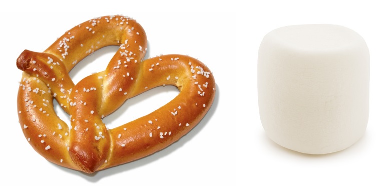
Walter Mischel’s marshmallow test was a milestone experiment in understanding the cognitive mechanisms of willpower. It goes in two parts – the initial experiments he and his team carried out in the late sixties and early seventies. The second part was establishing correlations of those test results with the test subject’s long term success in life. We will not go into the second part as, I suspect, it had a lot of subjective or potentially confounding effects, which is outside the simple realm of data analytics.

The paper published in 1972 in the Journal of Personality and Social Psychology, which follows up from his 1970 paper in the same journal, is the subject in today’s post. The objective of the test was to find out how young children (preschool kids, aged between 3.5 to 5.5 years) managed to delay the gratification of eating their favourite sweets under various experimental conditions. The neatness of the paper is that it doesn’t theorise a lot about cognitive abilities but rather gives data on how average children postponed their urge to eat (marshmallow or pretzel) under various distraction conditions.

There were three experiments in total; the first had five batches of children (total 50), the second (32) and the third (16) had three each.

The Task

Except for the last batch of three experiments, sweets were placed in front of the children. They had the option to eat their favourite sweet by calling the experimenter or win the second sweet (reward) if they had delayed gratification and waited until the experimenter came back. The experimenter recorded the time taken by each child before yielding to temptation. As the main variable, different distraction opportunities were given to the children. These are:

GroupObjective Distraction techniqueMean waiting time
1Wait for contingent reward (visible)Toy9 min
2Wait for contingent reward (visible) Think Fun12 min
3Wait for contingent reward (visible) None (control)< 1 min
4No contingent reward Toy (control)2 min
5No contingent reward Think Fun (control)1 min
6Wait for contingent reward (visible) Think Fun 13 min
7Wait for contingent reward (visible) Think Sad5 min
8Wait for contingent reward (visible) Think Rewards4 min
9Wait for contingent reward (hidden)No Ideation13 min
10Wait for contingent reward (hidden) Think Fun14 min
11Wait for contingent reward (hidden) Think rewards1 min

Summary

One startling finding was that children were willing to wait for a longer time when they were immersed in happy feelings, irrespective of whether the rewards were visible to them or not. Thinking about sweets and sad feelings were both unsuccessful in building willpower. The torture of thinking about the prize was no different from any other sad feelings!

The Marshmallow Test Read More »

Non-Zero-Sum Games

This post follows from an article titled “Keep on trucking”, published in The Economist.

Zero-sum games are templates hard-wired to our brains. We have seen a possible reason for this your-win-is-my-loss syndrome. The cognitive bias towards zero-sum thinking is sometimes called the fixed pie fallacy. Examples are everywhere – immigration, retirement ages, computerisation, outsourcing, the list is endless!!

Take, for example, the argument against the increase of retirement age. Part of the society, the younger lot, genuinely feel either their progress will stall or new opportunities will dry out due to the older generation keeping their jobs for longer.

The lump-of-labour fallacy, so it is known, is very appealing to everybody. But the data suggest something else. In developed economies, the higher employment rate of the old (55-64) is often positively correlated to a higher rate for the young (15-24). Reports of ILO can tell similar stories on migration – correlation between increased prosperity of the economy and the presence of migrant workers.

This fallacy appeals to most due to the simplistic picture it presents – a fixed amount of wealth that can only be exchanged between people, a form of the law of conservation of wealth. They conveniently forget human history. Wealth creation is the story of the modern world. Imaginative and innovative economies grew faster than inward-looking ones. Think about the cost to society when a person is retired. She no longer contributes but withdraws from public (pension) funds. In other words, part of the money from the younger lot goes out from the funds, built on bonds or equities, which could otherwise get more time to circulate and compound. On the other hand, if older people are still in the workforce, they spend, and money comes back to the economy, creating more (diverse types of) jobs that employ more, and the cycle continues.

The economies that kick part of their people out to employ the next batch are doing so either due to ignorance or because their economies are genuine candidates for zero-sum. Such economies are unlikely to prosper due to the same reason – the lack of imagination and growth mindset. We have ample examples to support from the last 300 years of human history.

Keep-on-trucking: The Economist

Non-Zero-Sum Games Read More »

How to Win Rock Paper Scissors

We continue the topic of zero-sum games and rock paper scissors. Winnie and Lucy have now decided to embark on a million-round game of rock paper scissors. They have done their preparations very meticulously, and they are ready. Let’s start following them with the simulations of their expected game and scores.

ti <- 0
win <- 0
luc <- 0

wr <- 1/3
wp <- 1/3
ws <- 1-wr-wp

lr <- 1/3
lp <- 1/3
ls <- 1-lr-lp

for (val in 1: 1000000){
Winnie <- sample(c("Rock", "Paper", "Scissors"), 1, replace = TRUE, prob = c(wr, wp, ws))
Lucy   <- sample(c("Rock", "Paper", "Scissors"), 1, replace = TRUE, prob = c(lr, lp, ls))
game_fin <- paste(Winnie = Winnie, Lucy = Lucy)


if (identical(Winnie, Lucy)) {
  #print("tie")
  ti <- ti + 1
  } else if(Winnie == "Rock" & Lucy == "Scissors" | Winnie == "Paper" & Lucy == "Rock" | Winnie == "Scissors" & Lucy == "Paper") {
  #print("Winnie Wins")
    win <- win + 1
  } else {
   #print("Lucy Wins")
    luc <- luc + 1
}

}


win * 100/ (win + luc + ti)
luc * 100/ (win + luc + ti)

W: 33.3; L: 33.3. If they both follow a random strategy, giving equal weightage to each of the three options, the expected results are a third for each outcome (win, loss, tie).


After about 1000 games, Lucy notices that Winnie have a slight bias towards the rock. Since she counted hands, Lucy thinks it is around (1.2/3). Note that it did not affect the overall results, which is still at
W: 33.3
L: 33.3

Lucy sees the opportunity and adjusts her game. She increases the paper to 1.2 in 3 and starts to see the results in the next 1000 games.
W: 33.0
L: 34.0

She also reduced the proportion of scissors from her kitty and found that her winning margin increased slightly.
W: 32.7
L: 34.0

Lucy now knows that providing the paper with a higher chance (1.5/3) could fetch an even better margin, she, however, doesn’t attempt for it, suspecting Winnie would figure it out.

Lucy did not know that Winnie used to be the junior champion in her college days. Winnie was testing Lucy by giving the bait to change her from a random strategy to having a bias. Noting Lucy has changed to a more-paper-strategy, Winnie changes to a scissor biased game (1.2/3).
W: 34.0
L: 33.3

Lucy noticed it after about 1000 games. Now Lucy knows Winnie knows Lucy knows. Or strategy is getting common knowledge. She has only one way out. Go back to random. The outcome is back at 33.3% for both, irrespective of what Winnie did.

In Summary

The best strategy to win a game of rock paper scissors is that there are no strategies unless the opponent gives one. Otherwise, you stick to random choices and leave the results to randomness in the short run, or if you are on a day-long game, a likely stalemate.

How to Win Rock Paper Scissors Read More »

Zero-Sum Games

fingers, fist, hands-149296.jpg

Zero-sum game. We use a rock-paper-scissors game to explain a zero-sum game. The game is played between two players, in which the players simultaneously show a rock, paper or scissors, using hand gestures. The rule is: rock breaks scissors, scissors cut paper and paper covers rock. The winner gets one point, and the loser loses 1. If both show the same gesture, they get nothing. Let’s write down the payoff matrix (refer to game theory).

Winnie
RockPaperScissors
RockL = 0, W = 0L = -1, W = 1L = 1, W = -1
LucyPaperL = 1, W = -1L = 0, W = 0 L = -1, W = 1
Scissors L = -1, W = 1 L = 1, W = -1 L = 0, W = 0

So, Winnie’s loss can only come from Lucy’s win or vice versa. If they both show the same hand, the game offers no points. In other words, if you sum each of the cells in the table, you get zero. It is a zero-sum game.

Several games follow this pattern – grand slam tennis matches, football (soccer) games in the knockout stages, NBA, to name a few. Irrespective of how much or how little zero-sum games represent our real life, the notion is hard-wired in the brain thanks to popular culture (the good at the expense of the bad) or high profile presidential elections (Republicans’ loss is Democrats gain).

Sometimes, playing for a tie in the league phase of a football tournament can be a strategy for a team (or both teams) to advance to a playoff / knockout round. Similarly, coalition governments are real possibilities in several countries. These are all examples of win-win situations.

Zero-Sum Games Read More »

The Martingale Fallacy

Martingale appears a compelling strategy to make money from the Roulette game. In the Martingale technique, you make an even-money (bottom row of the layout) bet. If successful, you win a unit profit (payoff is 1 to 1); end of the story. If you fail, you stay for another spin but double the wager, and you continue this pattern until you win. The argument is that if you play the game infinitely, the chances of repeated failure reach zero. That is a correct argument.

The opposite is also true – if you are on a losing track, withdrawing from the game or continuing on a reduced bet than required will result in losses. And that is what the casino will do. They put bet limits, say, at 500 dollars. That means, once your wager reaches above 500, you got to stay at 500, suggesting a loss of money even if you win from there onwards.

I will start the illustration with the first bet and win.

Try Bet Outcome Spent Gained Profit
11WIN121

Imagine you lost the first spin, and as per Martingale strategy, you double the bet and continue at the same spot.

TryBetOutcomeSpentGainedProfit
11FAIL1
22WIN341

This doubling bets each time appears like you double the potential profit also. But in reality, you exactly get the starting unit. Here is the illustration of winning after eight successive rounds of failure.

TryBetOutcomeSpentGainedProfit
11FAIL1
22FAIL 3
34FAIL 7
48FAIL 15
516FAIL 31
632FAIL 63
764FAIL 127
8128FAIL255
9256WIN5115121

Once your doubling reaches above 500, you have to stay at 500, suggesting a loss of money even if you win from here onwards.

TryBetOutcomeSpentGainedProfit
11FAIL1
22FAIL 3
34FAIL 7
48FAIL 15
516FAIL 31
632FAIL 63
764FAIL 127
8128FAIL255
9256FAIL511
10500WIN10111000-11

You will argue that losing nine rounds in a row is highly unlikely. That is true; after all, the probability of staying on the losing course for nine spins is (20/38)9 = 0.3%.

That is why the motivation for playing the game is crucial. If it is for fun and making a dollar or two, this makes a perfect strategy. However, if you want to make money by this strategy, you will see the odds of getting nine successive fail is no smaller. Suppose the wheel spins 200 times the chance of nine failures in a row is one in three (see the earlier post for the calculations). The nightmare possibility can come on the 9th or the 600th.

The other argument is to start with more than 1 unit, as at the end of the day, one dollar starting bet will only get you 1 dollar as profit. Imagine you start with 5 dollars. The table is below.

TryBetOutcomeSpentGainedProfit
15FAIL5
210FAIL 15
320FAIL 35
440FAIL 75
580FAIL 155
6160FAIL 315
7320WIN6356405

The trouble with this is that you approach your ceiling in seven spins, and you lose 135 even if you win the 8th round. Now, the probability of getting seven consecutive fail in 200 games is almost certain (100%)! An extreme case is putting the first bet at 500. If you fail the first time, the game is no more any strategy, as you have only one chance to recover or lose 1000.

Martingale Strategy is Fun

It is a strategy to have fun, test your probability models and earn a few dollars but not get rich. The doubling of bets gives a feeling of doubling the profit, but we have seen that the final gain is always equal to the initial bet and higher the initial, you reach the ‘ceiling’ faster. If you continue the excitement after a few successes (1 or 2 dollars), the odds will hit you and take away everything.

The Martingale Fallacy Read More »

Probability of Streaks

You have seen the binomial theorem. If you toss a coin 7 times, what is the chance of seeing all heads? It’s (1/2)7 = 0.0078 – less than a 1% chance! Now, what is the chance of seeing 7 consecutive heads at least once if you toss 200 times?

Let’s run this R code on random sampling and do Monte Carlo simulations to average it over 10,000 instances of 200 coin tosses.

library(stringr)

trial <- 10000

streak <- replicate(trial, {
toss <- sample(c("H", "T"), 200, replace = TRUE, prob = c(0.5,0.5))
toss1 <- paste(toss,collapse=" ")
count <- str_count(toss1, c("H H H H H H H"))

})

mean(streak)

Chance is more than 75%

Ok, what is the chance of seven heads if the probability of heads is increased slightly to 20/38? Almost always. There is a reason for this strange-looking probability of 20/38. That is next.

Probability of Streaks Read More »

Chance of Having a Healthy Pair of Chromosomes

Here is a question. A lady has a brother who has haemophilia. Their parents did not have the disease, and her two sons also did not have any issues. What is the chance that the lady has a fine pair of X chromosomes? No other information.

Haemophilia is an inherited genetic disorder and is associated with X chromosomes. Typically, women have a low probability of having the condition as the likelihood of having errors in both the X chromosomes is low.

So, how do we work out the problem? The brother has haemophilia, which suggests that one X chromosome of their mother has the error. Why? Father can only give his Y to the son. Additionally, the father did not have the condition, suggesting his X was healthy. Now, the mother can pass the error or the error-free X to her daughter. So there are two chances: the lady has two healthy Xs (A) or one error X (notA). Since she has sons, their X must have come from her. The two children are unaffected (B).

The probability of two healthy sons if the lady has two healthy Xs, P(B|A) = 1. The chance of two healthy children if the lady has one unhealthy X, P(B|notA) is (1/2)x(1/2) = 1/4. P(A), the lady has healthy XX = (1/2) and P(notA), one unhealthy X = (1/2). We have everything. Call Mr Bayes.

The chance of the lady has a healthy XX, given that her two sons are healthy,

P(A|B) = \frac{P(B|A)  P(A)}{P(B|A) P(A) + P(B|notA) * P(notA)} \\ \\  = \frac{ 1  (1/2)}{1  (1/2) + (1/4)(1/2)} + \frac{ (1/2)}{(1/2) + (1/8)}  = 8/10

= 80%

Chance of Having a Healthy Pair of Chromosomes Read More »

Life in a Funnel

Random processes are far mischievous than you could ever imagine. It is partly due to the inability of our minds to correctly understand randomness in real life. Yes, it is easy to follow in classrooms – those head and tail stuff. If I toss a coin once, I get 100% of an outcome, irrespective of its theoretical probability of occurrence of 0.5, piece of cake! It is easy for us to acknowledge the gambler fallacy or the theory of large numbers.

Yet, when it comes to real life, especially when it comes to rare events, we forget all we have learned and become captains of the ship of irrationality. Today we take an example, which is the favourite of reporters and cherry-pickers.

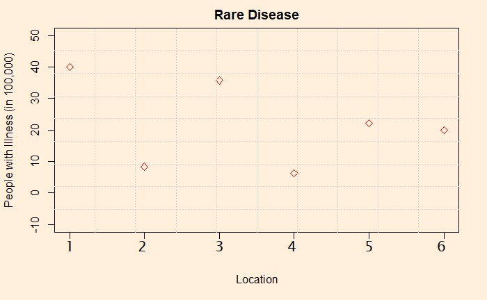
Consider this: you are working in the city centre, and want to live in one of its suburbs – place1. Your friend comes to know about your decision, and she shows you a newspaper article that talks about the stats on a rare disease. She recommends place2 or place4 as she thinks place 1 has four times more prevalence of the disease.

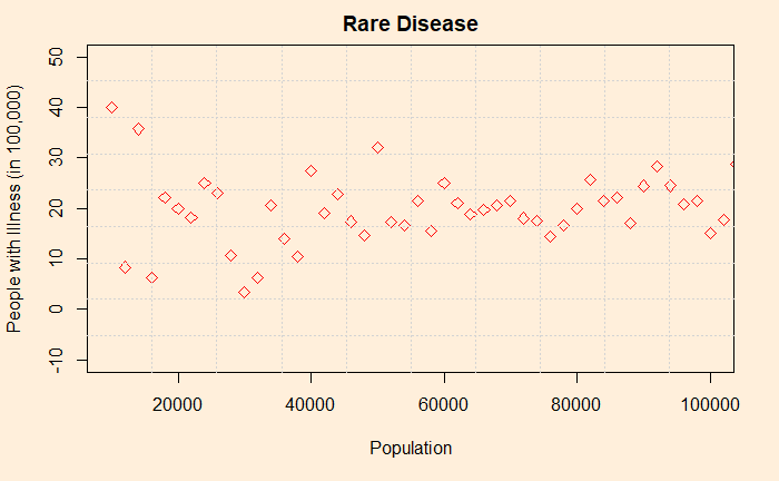
You are not happy, and you find out the population of those places – They are between 10,000 to 20,000. You then collect data on the disease from more parts of the world and find the following.

You are more interested now, and you refer to the standard statistics textbook and read about binomial trials. You make an assumption, based on the data points towards the right-hand side and decide that the mean value is 20 per 100,000 population. Then finds two formulae for random variables that followed binomial distributions (Bernoulli).

\text{expected value of } X, E(X) = p \\ \\ \text{where p the probability of success (in this case, the disease!)} \\ \\ \text{standard deviation of X } = \sqrt{ p q} \\ \\ \text{q = 1 - p, the probability of failure (no disease)}

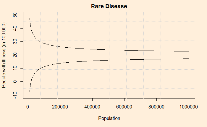
You assume E(X) to be 20/100,000 and patiently estimate the standard deviation and then standard error (by diving with the square root of population) for populations from 10,000 to a million. And generate a plot of a 95% confidence interval. Don’t know how to estimate confidence intervals? Check this out.

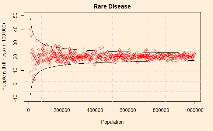
In the whole of this exercise, you used only a single number for the disease probability but got a funnel-like plot! Now you get more data from all over the world and they fit inside the funnel.

The incidence of disease enclosed in 95% confidence interval

What are your conclusions?

1) There is nothing wrong with any of those six places – at least regarding this rare disease.
2) People make the mistake of misinterpreting randomness in smaller populations all the time.
3) One reason is lack of knowledge.
4) The other reason is fundamental to our species; its complete surrender to two emotions – fear and greed. It was greed that made you a bankrupt chasing gambler fallacy. This time, it is the fear of disease, which made you forget your basics.

Further reading

The art of statistics: Learning from Data: David Spiegelhalter

Life in a Funnel Read More »

House Advantage

The rules of roulette appear complex, with so many types of bets and payoffs. We have seen the basic odds of roulette in an older post, and this time we spend time demystifying the complexity. First, look at the wheel (American roulette).

And the layout on which the player places the bet is:

Now, various possible bets and payoffs.

BetExplanationnumbers
covered
Payoff
Straightthe bet covers a number 135 to 1
Splitbet on two adjacent numbers on the layout217 to 1
Streetbet on a column of 3 numbers (e.g. 12, 11, 10)311 to 1
Cornerany block of 4 numbers of 2 x 2 (e.g. 32, 35, 31, 34)48 to 1
Basketfive number combination of 00, 0, 3, 2, 156 to 1
Double Street2 adjacent columns of the layout; a bet covers 6 numbers65 to 1
A dozen1-12, 13-24 or 25-36, by placing a bet on one of the 3 locations of the layout 122 to 1
Even-moneyodd/even, red/black, low (1-18), high (19-36)181 to 1

Now, forget everything and let’s find out how payoffs are made, and what the expected values are.

Expected Value, E

The expected value of a random variable is a weighted average. In other words, you take the value of each variable, multiply it by its probability to occur and sum over all the variables. Imagine a coin-tossing game – you get one dollar for a head and lose 1 for a tail. The outcomes hear and tails, are random variables, each with a chance of 1 in 2 (0.5). So, the expected value = P(H) x V(H) + P(T) x V(T) = (1/2)x(1) + (1/2)(-1) = 0. Or, if you play the game over and over, you are expected to gain (or lose) nothing, but you should play for a long time to see that outcome. I have used V to denote value.

Another example: you play 6-sided dice. You get 6 dollars if the dice rolls on 3, and lose 1 dollar for everything else. The expected value (if you play long enough) is E = (1/6)(-1) + (1/6)(-1) + (1/6)(6) + (1/6)(-1) + (1/6)(-1) + (1/6)(-1) = (6/6) – (5/6) = 1/6. So, keep playing.

Roulette

We have seen how it works in Casino games. We will formalise it this time. Look carefully at the last two columns of the bet-payoff table, and you can make a formula payoff = (36 – numbers covered ) / numbers covered. The formula holds good except for Basket, where the answer is (36-5)/5 = 6.2, but the casino rounds it off to 6 (benefits who?).

Let N be the number of pockets on the wheel (38 for American and 37 for European), and n be the number covered. The chance of getting one number from 38 possibilities is (1/38). The probability of getting one out of two numbers (such as a split) is (1/38) + (1/38) = 2/38 – remember the addition rule of mutually exclusive events? So the generalised formula for getting one number in a bet that covers n numbers is n/38, and the expected value is

E = \frac{n}{N}*\frac{36 - n}{n} + (-1)*\frac{N-n}{N} \\ \\ = \frac{(36 - n - N + n)}{N} = \frac{(36 - N)}{N}

There is something special about the final equation – that it is independent of the numbers covered but depends only on the number of pockets on the roulette wheel. In other words, if the game has a smart payoff structure given by a formula (36 – numbers covered ) / numbers covered, you get a bet-independent payoff (or a constant payoff).

House wins, always

We will plug in numbers and find out the advantage – you already know it’s a house advantage for any N more than 36. So for the American, it is (36-38)/38 = – 0.0526 or 5.26%; for the European, it is (36-37)/37 = – 0.027 or 2.7%. The Basket doesn’t exactly fit the rule, and its house advantage is higher at 7.89%.

House Advantage Read More »