Data & Statistics

Expert’s Curse 1: Base Rate Fallacy

The first one on the list is the base rate fallacy or base rate neglect. We have seen it before, and it is easier to understand the concept with the help of Bayes’ theorem.
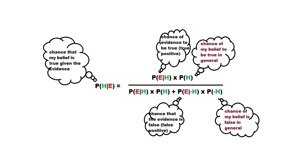
P(H) in the above equation, the prior probability of my hypothesis on the event is the base rate. For the case study of doctors in the previous post, the problem starts when the patient presents a set of symptoms. Take the example of the case of UTI from the questionnaire:

Mr. Williams, a 65-year-old man, comes to the office for follow up of his osteoarthritis. He has noted foul-smelling urine and no pain or difficulty with urination. A urine dipstick shows trace blood. He has no particular preference for testing and wants your advice.

eAppendix 1.: Morgan DJ, Pineles L, Owczarzak, et al. Accuracy of Practitioner Estimates of Probability of Diagnosis Before and After Testing. Published online April 5, 2021. JAMA Internal Medicine. doi:10.1001/jamainternmed.2021.0269

The median estimate from the practitioners suggested that they guessed a one-in-four probability of UTI (ranging from 10% to 60%). In reality, based on historical data, such symptoms lead to less than one in a hundred!

Was it only the base rate?

I want to argue that the medical professionals made more than one error, i.e., base rate neglect. As evident from the answer to the last question, it could be a combination of two possible suspects—anchoring and the prosecutor’s fallacy. First, let’s look at the questions and answers.

A test to detect a disease for which prevalence is 1 out of 1000 has a sensitivity of 100% and specificity of 95%.

The median survey response was 95% post-test probability (in reality, 2%!) for a positive and 2% (in reality, 0) for a negative.

The prosecutor’s fallacy arises from the confusion between P(H|E) and P(E|H). In the present context, P(E|H), also called the sensitivity, was 100%, but the answers got anchored to 95% representing specificity. To understand what I just meant, look at the Bayes’ rule in a different form:

\\ \text{Chance of Disease after a +ve result} = \frac{Sensitivity *  Prevalence}{Sensitivity *  Prevalence + (1-Specificity)*(1- Prevalence)} \\ \\ \text{Chance of Disease after a -ve result} = \frac{(1- Sensitivity )*  Prevalence}{(1- Sensitivity )*  Prevalence + Specificity*(1 - Prevalence)}

So it is not a classical prosecutor’s case but more like getting hooked to 95%, irrespective of what it meant—it is more of a case of anchoring.

Expert’s Curse 1: Base Rate Fallacy Read More »

The Curse of Expertise 

Practitioners are experts. They could be medical practitioners, domain experts, lawyers and judges, leaders of organisations, sports persons-turned-pundits, to name a few. A lot of decision making rests on their shoulders, and the tool they often employ is experience. And experience is a double-edged sword! On the one hand, it makes them the most suitable people for the job, but on the other hand, they tend to ignore quantitative inference and rely on personal experience instead.

JAMA Internal Medicine collected responses from 723 practitioners from outpatient clinics in the US and published a paper in April 2021. The study aimed to estimate the understanding of risks and clinical decisions taken by medical practitioners. They included physicians and nurse practitioners. They were given a questionnaire to fill in the pretest and post-test probabilities of a set of illnesses. The requested post-test estimates included those after positive tests and negative tests.

The survey had five questions – four containing clinical scenarios (pneumonia, breast cancer, cardiac ischemia and UTI) and one hypothetical testing situation (a disease with 0.1% prevalence and test with 100% sensitivity and 95% specificity). The scientific evidence and the median responses are tabulated below:

Clinical
Scenario
Scientific
evidence
Estimate
Resident
physician
Estimate
attending
physician
Estimate
Nurse
practitioner
Pneumonia
pretest
probability
25-42808580
post-test
after +ve test
46-65959595
post-test
after – ve test
10-19605050
breast cancer
pretest
probability
0.2 – 0.35210
post-test
after +ve test
3 – 9605060
post-test
after – ve test
< 0.055110
cardiac ischemia
pretest
probability
1-4.410515
post-test
after +ve test
2-11756090
post-test
after – ve test
0.43-2.55510
UTI
pretest
probability
0-1252030
post-test
after +ve test
0-8.377.59090
post-test
after – ve test
0-0.11555
Hypothetical
Scenario
post-test
after +ve test
2959595
post-test
after – ve test
0255

Those unheard are …

Before pointing fingers at the medical practitioners: you get this data because someone cared to measure, the specialists were happy to cooperate, and the Medical Association had the courage and insight to publish it. And the ultimate objective is quality improvement.

At the same time, the survey results suggest the lack of awareness of the element of probability in clinical practice and call for greater urgency to focus on scientific, evidence-based medical practice.

Morgan et al., JAMA Intern Med. 2021;181(6):747-755

The Curse of Expertise  Read More »

Hazard ratio and Chilli Magic

Clinical trials describe study results, which are essentially time-to-event data on risks, followed systematically from the standpoint of an event of interest, using the term Hazard Ratio (HR). HR gives the comparison of two risks positioned side by side on a survivorship plot. A survival plot can represent the number of people remaining alive in the study period, the time to disappear a pain, the time to recover from a disease in the presence of an intervention drug and so on.

Kaplan – Meier plot is a curve with time on the x-axis, and the proportion (or number) of people surviving is on the y-axis. For estimating the HR, the Kaplan – Meier plot should have two curves – one representing the intervention (experimental) group and the other the control (placebo) group.

Chilli pepper study

The famous 2019 paper on chilli pepper is an example to illustrate the hazard ratio. The researchers have followed a group of 22811 for about eight years and recorded the survival plot. The group had 15122 chilli eaters (experimental group) and 7689 non-chilli eaters (control group). A total of 1236 people had died by the end of the study, of which 500 were non-chilli eaters, and 736 were chilli takers. Let’s calculate:

Risk of death for chilli eaters = 736 / 15122
Risk of death for non chilli takers = 500 / 7689
The ratio = (736 / 15122) / (500 / 7689) = 0.75.
We will call the ratio the hazard ratio (HR) for the chilli eaters.

When the team looked at the specific cause of death, Cardiovascular disease (CVD), they found the following:

Risk of CVD mortality for chilli eaters = 251/ 15122
Risk of CVD mortality for non chilli takers = 193/ 7689
Hazard ratio = (251/ 15122) / (193/ 7689) = 0.66

So what are you waiting for? Eat your chilli and postpone the eventuality!

Bonaccio et al., Journal of the American College of Cardiology, 7 4 (25), 2019

Kaplan – Meier estimator: wiki

Hazard ratio and Chilli Magic Read More »

Risk ratio and Odds Ratio

What is the risk of you getting lost in the barrage of jargon used by statisticians? What are the odds of the earlier statement being true? Risks, odds and their corresponding ratios are terms used by statisticians to mesmerise non-statisticians.

Risk is probability, p

In medical studies, the phrase risk means probability. For example: if one person has cancer in a population of 1000 people, we call the risk of cancer in that society is (1/1000) or 0.001. For coin flipping, our favourite hobby, the risk of having a head is (1/2) = 0.5, and for rolling a dice, the risk of getting a 3 is (1/6) or 0.167. You may call it the absolute risk because you will see something soon that is not absolute (called relative), so be prepared.

Odds are p/(1-p)

Odds are the probability of an event occurring in a group divided by the probability of the event not occurring. Odds are the favourite for bettors. The odds of cancer in the earlier fictitious society are (1/1000)/(999/1000) =0.001. The number appears similar to the risk, which is only a coincidence due to the small value of the probability. For coin tossing, the odds of heads are (0.5/0.5) = 1, and for the dice, (0.167/0.833) = 0.2. Conversely, the odds of getting anything but a 3 in dice is (5/6)/(1/6) = 0.833/0.167 = 5.

Titanic survivors

SexDiedSurvivedRisk
Men13643671364/(1364+367)
0.79
Women126344126/(126 + 344)
0.27
SexDeathSurvivalOdds
Men0.791-0.790.79/(1-0.79)
3.76
Women0.271-0.270.27/(1-0.27)
0.37

The risk shuttles between 0 and 1; odds, on the other hand, it is 0 to infinity. When the risk moves above 0.5, the odds crosses 1.

Now, the ratios, RR and OR

Risk Ratio (RR) is the same as Relative Risk (RR). If the risk of cancer in one group is 0.002 and in another is 0.001, then RR = (0.002/0.001) = 2. The RR of losing dice rolling to coin tossing is (5/6)/(1/2)= 1.7. In the titanic example, the RR (between men and women) is (0.79/0.27) = 2.93.

The Odds Ratio (OR) is the ratio of odds. The odds ratio for titanic is (3.76/0.37) = 10.16.

Risk ratio and Odds Ratio Read More »

When Mother Became Nature

Sexual selection is a topic that invoked some controversy among evolutionary biologists. Darwin distinguished sexual selection as the difference in the ability to produce offspring, and natural selection, on the other hand, is about the struggles for existence.

Sexual selection is a combination of many factors. It could be a male-male struggle to reach a female, females snubbing males with certain features, or simply mating with certain males leading to weaker or no offspring.

mtDNA and NRY know it all

Whatever may be the precise reason, it has been established now using complex DNA analysis and computation that historically, more females and fewer males have participated in the development of the human race. In other words, throughout human history, leave the modern time when females started moving with their partners, fewer men participated in the reproduction process, although there are no reasons to believe that their respective numbers in the population were different. It went to such a low around 8000 years ago when the female-to-male effective population ratio was about 17!

References

Lippold et al. Investigative Genetics 2014, 5:13, Human paternal and maternal demographic histories: insights from high-resolution Y chromosome and mtDNA sequences

Genome Res. 2015 Apr; 25(4): 459–466, A recent bottleneck of Y chromosome diversity coincides with a global change in culture

When Mother Became Nature Read More »

What the Eyewitness saw

We have seen earlier that much of the evidence, depending on the nature, gives only moderate separation of the probability distributions of guilty and innocent curves. Evidence from the eyewitness is a leader that plays a pivotal role in the trial process. The pioneering work of Elizabeth Loftus reveals a lot about the fallibility of memory and the malleability of the brain by misinformation.

It’s in the wording

The first one is on people’s ability to estimate. In one experiment, the participants were asked to guess about the height of a basketball player. One group was asked: “how tall was the player” and the other, “how short was”. The ‘tall’ group estimated a higher number on an average than the ‘short’; the height difference between the tall to short was about 15 mm!

In the second experiment, 100 students were shown a video involving motor accidents and asked a few questions in which 6 were test questions – three of them about what happened in the movie and three that did not. Half of the subjects were given questions that were framed using ‘a’, such as Did you see a …? The other half were asked using ‘the’, such as Did you see the …? An overwhelmingly more number of people responded yes to the ‘the’ questions than the ‘a’ queries, irrespective of whether those events happened in the movie or not.

The role of presupposition

It is about asking one question followed by a second one. The purpose of the first question is to plant some seeds in the participant to influence the subsequent one. Forty undergraduates at the University of Washington were shown a 3-min video taken from the film “diary of a student revolution”. In the end, they were given a questionnaire with 19 filler questions and one key question. Half of the people got the question: “was the leader of the four demonstrators a male?” and the other half “was the leader of the twelve demonstrators a male?”. A week later, the subjects were back to answer 12 questions in which one key question was “how many demonstrators did you see in the movie”. The people who were asked “12” gave an average of 8.85 as the answer, whereas the “4” gave 6.4.

And the result?

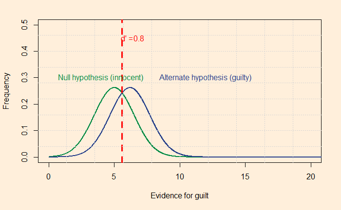
The results make descriptions by witnesses one of the least reliable forms of evidence to separate guilty from the innocent. Do you remember the d’ of 0.8 from the earlier post?

Loftus, E. F., Cognitive Psychology 7, 560-572

Elizabeth Loftus: Wiki

What the Eyewitness saw Read More »

Justice and the Use of Prior Beliefs

The last two posts ended with rather pessimistic notes on the possibility of establishing justice under the complex world of overlapping pieces of evidence. We end the series with the last technique and check if that offers a better hope of overcoming some inherent issues of separating signals from noise using the beta parameter.

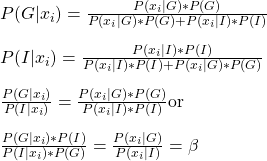
Beta comes from signal detection theory, and it is the ratio of likelihoods, i.e. P(xi|G)/P(xi|I). P(xi|G) is the probability of the evidence, given the person is guilty, and P(xi|I), if she is innocent.

Let us start from Bayes’ rule,

\\ P(G|x_i) = \frac{P(x_i|G)*P(G)}{P(x_i|G)*P(G) + P(x_i|I)*P(I)} \\ \\  P(I|x_i) = \frac{P(x_i|I)*P(I)}{P(x_i|I)*P(I) + P(x_i|G)*P(G)} \\ \\  \frac{P(G|x_i)}{P(I|x_i)} = \frac{P(x_i|G)*P(G)}{P(x_i|I)*P(I)} \text{or} \\ \\ \frac{P(G|x_i)*P(I)}{P(I|x_i)*P(G)} = \frac{P(x_i|G)}{P(x_i|I)} = \beta

So, beta depends on the posterior odds of guilt and the prior odds of innocent.

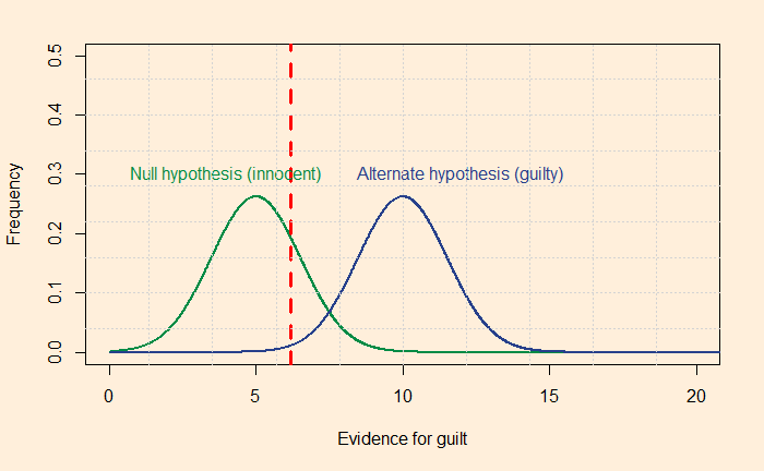
For a situation at a likelihood ratio of 1, if the prior belief, P(G), is lower, the jury is less likely to make a false alarm. Graphically, this means moving the vertical line to the right and achieving higher accuracy in preventing false alarms (at the expense of more misses).

The sad truth is that none of these techniques is helping to reduce the overall errors in judgement.

Do juries meet our expectations?: Arkes and Mellers

Justice and the Use of Prior Beliefs Read More »

Elusive Justice

We have seen perceived culpability vs probability distribution of evidence and their overlapping nature in the last post. It offers a simple picture, but the message demonstrates the difficulties of establishing justice for all. Today, we will go a step deeper by invoking signal detection theory, a strategy that can help detect signals from noise.

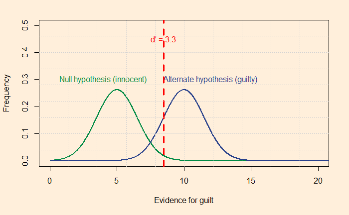
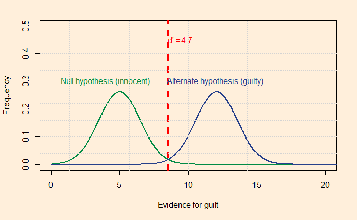
One technique to raise the level of justice (reduce misses and false alarms) is to increase the distance between the distribution curves from each other. Let’s look at it quantitatively: imagine you want not more than 5% misses and 5% false alarms, then the separation required between the two curves should be something like the following picture.

The red dotted line passes through the point on the 95th quantile of the green curve (calculated by the R formula, qnorm(0.95, 5, 1.52), where five is the mean and 1.52 is the standard deviation). You already know the meaning of 95% – it is 1.64 standard deviations away from the mean (equivalent to the one-sided confidence interval). The line also should match the left 5% of the blue curve (qnorm(0.05, 10, 1.52). One way to quantify the separation is to estimate the distance between the two distributions as a function of the standard deviation of the innocent.

d' = \frac{\mu_g - \mu_i}{\sigma_i} \\ \\ \mu_g \text{ = mean of guilty, }\mu_i \text{ = mean of innocent, and } \sigma_i \text{ = standard deviaton of innocent}

For the above plot, the separation is 3.3 standard deviations. If you wanted to see a more just system with a maximum of 1% errors, you need a detachment of 4.7.

Are 3.3 and 4.7 realistic?

Unfortunately, the answer is no! Look at some indicators that experimentalists have found out. For spotting lie, the d’ values obtained by studies stand at 0! d’ ranged from 0.6 to 0.9 for the polygraph test; the best-in-class gave close to 2.5, but that was exceptional.

Then come eyewitnesses: researchers did a meta-analysis of 120 studies and found d’ values of 0.8 on facial identification. Following is how d’ = 0.8 appears.

Medical tests have typically higher levels of d’ values but fall short of 3 (CT scans 3.0, mammograms 1.3 etc.), suggesting getting a 5% error level is a target difficult to achieve. What more can we do? We will see next.

Do juries meet our expectations?: Arkes and Mellers

Rationality: Steven Pinker

Elusive Justice Read More »

Justice for All

We all like to see justice happening in every trial. What is justice? In simple language, it is the conviction of the guilty and the acquittal of the innocent. In the court, jurors encounter facts, testimonies, arguments in support and against the defendant. The number and variety of evidence make them feel like random, independent events and make the hypothesis (that the accused is guilty or not) in front of the judge a distribution!

Overlapping Evidence

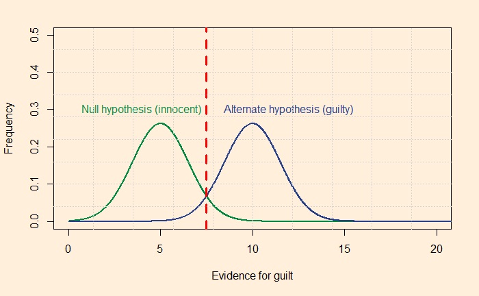
To illustrate the complexity of decision making, see the following two distributions (I chose uniform distribution as an example).

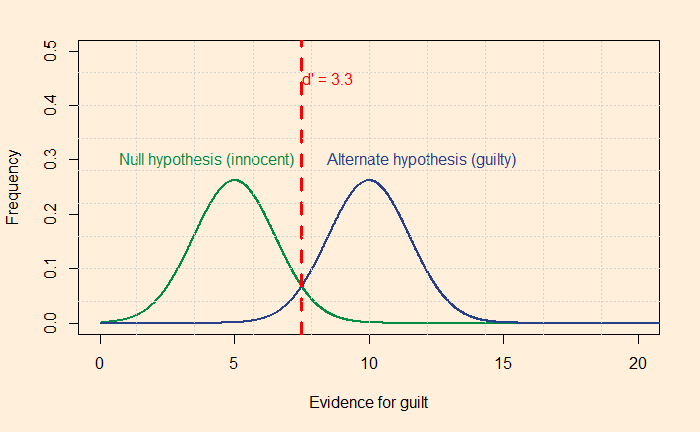
You can imagine four possibilities formed by such overlapping curves. The right-hand side tail of the innocent line (green) that enters the guilty (blue) region leads to the conviction of the innocent. The opposite – acquittal of the guilty – happens for the left-hand side tail of the guilty line that enters the non-guilty. The dotted line at the crossover of the two curves represents the default position of the decision or the point of optimal justice. At that junction, there are equal frequencies for false alarms and misses.

10 guilty for 1 innocent

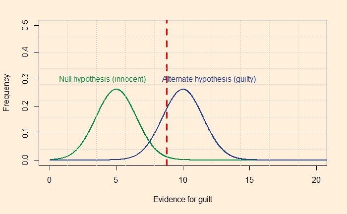
If the judge believes in Blackstone’s formulation, she will move her position to the right, as in the following plot.

The jury is willing to miss more guilty but assure fewer innocents are convicted. The opposite will happen if there is a zero-tolerance policy for the guilty; the examples in the real world are many, especially when it comes to crimes against national interest.

Errors and mitigations

So, what can jurors do to reduce the number of errors? We will look at more theoretical treatments and suggestions in the next post.

Do juries meet our expectations?: Arkes and Mellers

Justice for All Read More »

Binomial-Beta

Shaquille’s story continues. Last time, we made assumptions about each other’s feelings (hypotheses is the polished word!) for Shaq’s chance to enter the White House. Those assumptions were arbitrary: 0.9 and 0.2 for the probability of success or p. What about other factions? There are infinite of them between 0 and 1. This time, we will make no assumptions and take as many as possible using a continuous hypothesis generator.

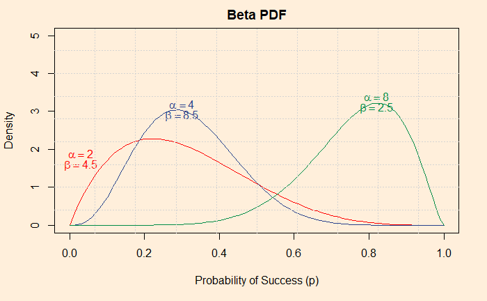
For that purpose, we will use the beta distribution function. Why beta? There is a reason for that, but we will know only towards the end. For now, we focus on what it can do for us more than what beta is. The beta distribution function can give a wide variety of probabilities for the entire range of p values. See three typical types (beta pdf uses two characteristic parameters, alpha and beta):

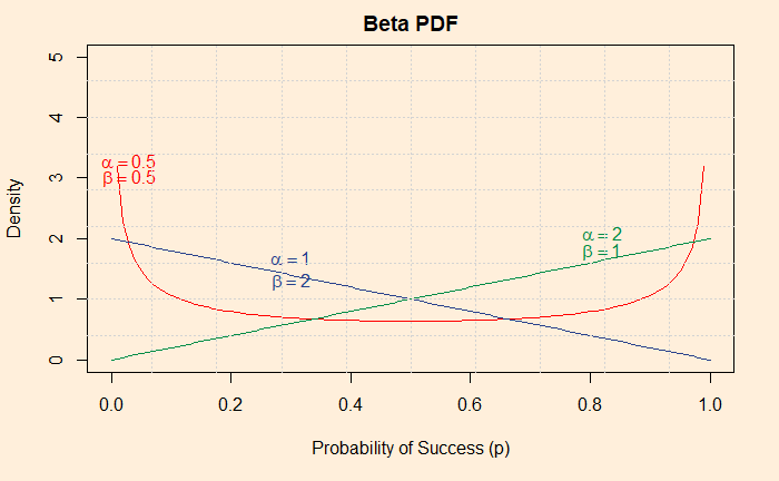
And three variety types:

The first reason to choose the beta distribution function (don’t get confused; this is not a beta function, which is a different beast) is that it takes the range of hypotheses (p) we are after as its input. i.e. 0 to 1.

What should Shaq and his friend choose?

Remember, Shaq and his friend have strong views about getting inside the White House, and they are betting! So, which shape of the beta distribution function should they choose? They are unlikely to use more consensus-driven types, the curves that bulge in the middle. Who will bet when two opinions are towards a single idea? So, they chose alpha = 0.5 and beta = 0.5 as their prior hypothesis.

Bayes’s to help after the misadventure

We know what happened: Shaq failed to get inside without the prior appointment, so the outcome was zero success in the first attempt. Now, we predict what happens if he tries again (without actually doing and finding it). That is where Bayesian inference comes in handy. That is also the second reason for choosing the beta distribution function. Write down the Bayes’ rule here, i.e. posterior = likelihood x prior / sum of all possibilities. In the world of continuous functions, integrations replace additions.

\\ beta(\alpha_{posterior}, \beta_{posterior} | data) = \frac{likelihood * beta(\alpha_{prior}, \beta_{prior}) }{\int likelihood * beta(\alpha_{prior}, \beta_{prior})} \\ \\ \text{likelihood is binomial distribution function, as seen in the previous post} \\\\ \text{likelihood} = f(s; n,p) = \binom{n}{s} p^s (1-p)^{n-s}

Then a miracle happens: a complicated equation applied over the prior beta function results in a posterior beta function with a few minor modifications. The posterior is:

\\ beta(\alpha_{posterior}, \beta_{posterior}) = beta(\alpha_{prior + s}, \beta_{prior + n - s}) \\ \\ \text{in the present case} \\ \\ beta(\alpha_{prior}, \beta_{prior}) = beta(0.5,0.5) \\ \\ beta(\alpha_{posterior}, \beta_{posterior}) = beta(0.5 + 0, 0.5 + 1 -0 ) = beta(0.5, 1.5) \\ \\

New betting scheme

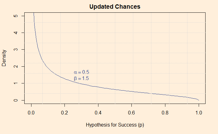
You know why s was zero and n was one, because Shaq did one (n) attempt and failed (s)! How does the new scenario, beta(0.5, 1.5), look? Here is the shape of beta(0.5, 1.5):

Putting together

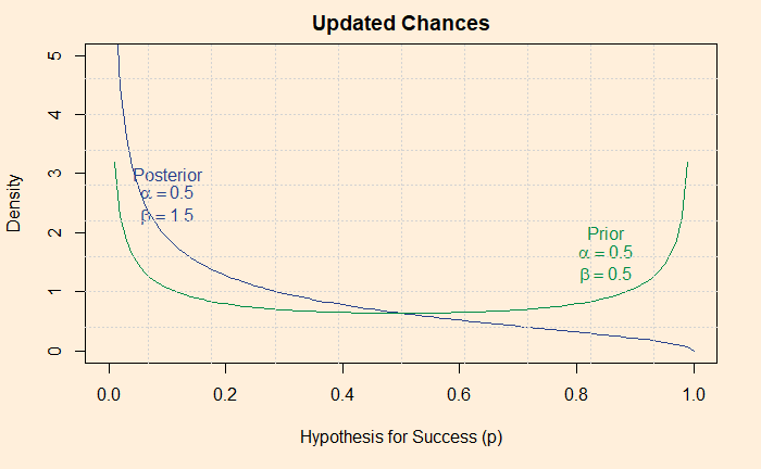
The updated chance of Shaq getting inside the White House has come down after the information that he failed in his first attempt came out.

Shaq Denied Entrance: Washington Post

Bayesian Statistics for Beginners: Donovan and Mickey

Binomial-Beta Read More »