Data & Statistics

Hypothesis Testing – Chi-Squared

The following table lists the weights of 50 boys (6-year-olds) sampled randomly. Can you test the hypothesis that the weights of 6-years old boys follow a normal distribution with a mean = 25 and a standard deviation = 2? We will do a chi-squared test to find out the answer to this.

2824272427
2625292224
2325212225
2627272629
2827222321
2924232322
2522292830
2428262525
2829262730
2231252427

The hypotheses

The null hypothesis, H0, in this case: there is no difference between the observed frequencies and the expected frequencies of a normal distribution with mean = 25 and standard deviation = 2.

The alternative hypothesis, HA: there is a difference between the observed frequencies and the expected frequencies of a normal distribution with mean = 25 and standard deviation = 2.

Estimation of chi2

Let us divide the data in the previous table into six groups of equal ranges. The frequencies of those ranges are counted. The expected frequency is estimated from the cumulative distribution function of the normal distribution for each of the ranges using the formula

Ei = n x [F(Ui) – F(Li)]

n is the number of samples, F(Ui) is the upper limit of a range, and F(Li) is the lower limit.

RangeObserved
Frequency (O)
Expected
Frequency (E)
(O-E)2/E
20 – 2120.831.65
22 -23106.651.69
24 -251316.450.72
26 – 271216.071.03
28 – 29106.212.31
30 – 3130.944.51
11.92

The critical value at the 5% significance level and the p-value are estimated using the following R code.

qchisq(0.05, 5, lower.tail = FALSE)
pchisq(11.92, df=5, lower.tail=FALSE)

The critical value is 11.07, and the p-value is 0.036. Since the estimated chi-square (11.92) is outside the critical value, we reject the null hypothesis that the data follow the normal distribution with a mean = 25 and a standard deviation of 2.

Hypothesis Testing – Chi-Squared Read More »
Chi-square for Independence

Another application of the chi-square statistics is to test for independence, applied to categorical variables. For example, if you did sampling and wanted to know the gender dependence on higher education. Following is the data collected.

MaleFemale
No Graduation76
College1613
Bachelors1516
Masters118

Test for Independence

You perform a chi-square to test for independence.

Male
Observed
Female
Observed
Total
No Graduation7613
College161329
Bachelors151631
Masters11819
Total494392
Observed Data

The expected data for a perfectly independent scenario is calculated as below. The expected value at (row i, column j) is obtained by RowSum(i) x ColumnSum(j)/(Grand Total).

Male
Expected
Female
Expected
Total
No Graduation13×49/92
= 6.92
13×43/92
= 6.08
13
College29×49/92
= 15.45
29×43/92
= 13.55
29
Bachelors31×49/92
= 16.51
31×43/92
= 14.49
31
Masters19×49/92
= 10.12
19×43/92
= 8.88
19
Total494392
Expected Data

The Chi-square is calculated as

Male
(O-E)2/E
Female
(O-E)2/E
Chi2
No Graduation(7-6.92)2/6.92
= 0.00092
(6-6.08)2/6.08
= 0.00105
College(16-15.45)2/15.45
= 0.0196
(13-13.55)2/13.55
= 0.0223
Bachelors(15-16.51)2/16.51
= 0.138
(16-14.49)2/14.49
= 0.157
Masters(11-10.12)2/10.12
= 0.0765
(8-8.88)2/8.88
= 0.087
Total0.2350.2680.503
Chi-square

Like, we have done previously, plug in the value for the 5% significance level (0.05) in R function qchisq with degrees of freedom 3. The answer is 7.81, which is the critical value. The calculated value of 0.503 is lower than 7.81, and therefore, the null hypothesis that education level is independent of gender can not be rejected. The p-value can be calculated by using 0.503 inside the R function, pchisq. The answer is 0.918.

qchisq(0.05, 3, lower.tail = FALSE)
pchisq(0.503, df=3, lower.tail=FALSE)

The R code for the whole exercise

edu_data <- matrix(c(7, 16, 15, 11, 6, 13, 16, 8), ncol = 4 , byrow = TRUE)
colnames(edu_data) <- c("no Grad", "College", "Bachelors", "Masters")
rownames(edu_data) <- c("male", "female")

chisq.test(edu_data)

Chi-square for Independence Read More »

Chi-Square Test for the Lefties

Randomness and the subsequent scattering of data can confuse people interpreting observations. Take this example: from studies, we know that 10% of the population is left-handed. You surveyed 150 people (randomly selected) and found that 20 are left-handed. Does this violate the theory, or it’s just normal? What do we do?

Goodness of fit

You perform a chi-square goodness of fit test on the data.

Observed (O)Expected (E)(O-E)2/E
Left 201525/15
Right13013525/135
Total1501501.85

We will reject the notion (that 10% is left-handed) with a 5% significance level. In other words, the evidence shall be outside the 95% confidence interval to support the alternative hypothesis. In our case, the alternative hypothesis is that the proportion of lefties is more than 10% of the population. So how do you estimate the critical value at a 0.05 (5%) significance level? In an old-fashioned way, there is a lookup table where you find out the number by matching the degrees of freedom (in this case, df = 1) and the significance level. We use the following R code to get it.

qchisq(0.05, 1, lower.tail = FALSE) # qchisq(p, df)

The answer is 3.84. In other words, the calculated value of the chi-squared needs to be greater than 3.84 to be outside the range to reject the notion (or the null hypothesis). In our case, it is 1.85, which is less than 3.84, and we can’t reject the notion of 10% lefties, although we see 20 in 150!

p-value

How to calculate our favourite p-value from this? For that, we plug in the chi-square value (1.85) in the pchisq function.

pchisq(1.85, df=1, lower.tail=FALSE)

The answer is 0.1737. Needless to say, pchisq is the inverse of qchisq. In other words

qchisq(0.1737, 1, lower.tail = FALSE)

gives 1.85.

Everything in one step

The following R code will do everything from the start

obsfreq <- c(20,130)
nullprobs <- c(0.1,0.9)
chisq.test(obsfreq,p=nullprobs)

The answer will be in the following format

	Chi-squared test for given probabilities

data:  obsfreq
X-squared = 1.8519, df = 1, p-value = 0.1736

Chi-Square Test for the Lefties Read More »

Expectations of a Random process

Gambler’s fallacy is the belief that a random process is somehow self-correcting. The word, somehow, is important here to note as you know that it is a random process and has no brain to self-correct! Check this out:

“The mean IQ of children in a city is 100. You take a sample of 50 children for a study. If the first child measures an IQ of 150, what is the expected average IQ of the group?”

Tversky and Kahneman, Psycological Bulletin, 1971

The answer is (150 + 49 x 100) / 50 = 101, althoght most people thought it would still be 100.

Another famous example is the hot hand in basketball. It is a belief from the spectators that a person’s success for a basket depends on previous success. But a lot of studies have not found any evidence for such dependencies.

Expectations of a Random process Read More »

When We Start Predicting Randomness

The answer to the birthday problem comes as a surprise to most of us. If you have not heard about this puzzle, you may read one of my earlier posts. At the same time, it is far less controversial than, say, the Monty Hall problem, as the former can be solved mathematically without much ambiguity.

A similar story on a Canadian lottery is narrated in the book The Drunkard’s Walk: How Randomness Rules Our Lives by Leonard Mlodinow. The officials have decided to give away 500 cars to 2.4 million of its subscribers using the unclaimed prize money of the past. They used a computer program to randomly pick 500 individuals and published the unsorted results, obviously not aware of the possibility of double-counting. And the result? One number was repeated, and a person got the car twice!

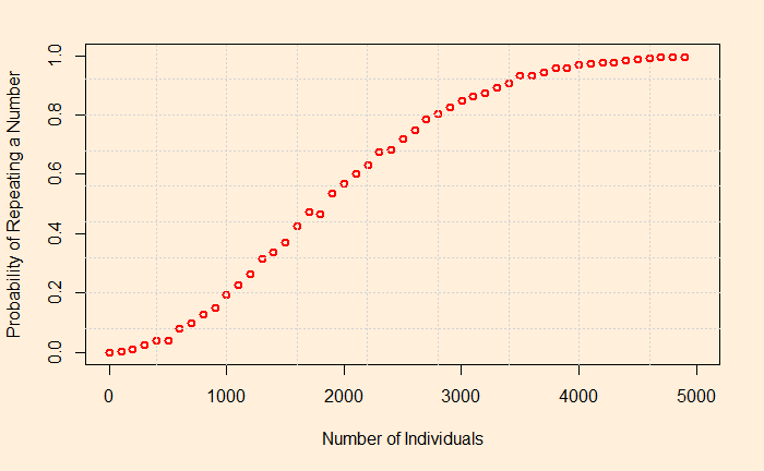
Let’s write an R code to numerically understand the probability of such an event to happen – a repeat of a number within 500, spread over 2.4 million. The program repeats a random number generation (the sample function), 500 at a time, 10000 times and averages it.

B<- 10000
n<- 500

results<- replicate(B, {
  lot<- sample(1:2400000, n, replace=TRUE)
  any(duplicated(lot))
})
mean(results)

The program output, the probability of a repeat inside 500 numbers, is 5.4% – not an infinitesimally small number by any standard. The following plot shows how it grows with the sample size.

You will see that the repeat is almost certain before the number reaches about 4000.

When We Start Predicting Randomness Read More »

Probability of Defective Coin

You suspect that one of the 100 coins in a bag is 60% biased towards heads. You take one coin at random, flip it 50 times and get 30 heads. What is the probability that the coin you chose is biased?

Let’s do this Bayesian challenge step by step. Let B = biased, nB = not biased, and D = outcome (data). The probability that the coin is biased, given the data of 30 heads out of 100 flips,

\\ p(B|D) = \frac{P(D|B)*P(B)}{P(D|B)P(B) + P(D|nB)*P(nB)}

The likelihood, P(Data|B)

The first term of the numerator is called the likelihood. What is the likelihood of getting 30 heads in 50 flips if the coin is biased 60%? We know how to get that quantity – apply a binomial trial with a chance of 0.6 for success and 0.4 for failure. The term in the denominator, P(D|nB)*P(nB), the probability of 30 heads if the coin is not biased, means you make success and failure at 0.5.

Since you have the information that 1 in 100 coins is faulty, you chose 1/100 as the prior knowledge. The R code of the calculation is given below.

head_p <- 0.6
tail_q <- 1 - head_p
prior <- 1/100

flip   <- 50
success_head <- 30

prob_bias <- choose(flip, success_head)*(head_p^(success_head))*(tail_q^(flip-success_head))  

head_p <- 0.5
tail_q <- 1 - head_p
prior_no <- 1 - prior
prob_no_bias <- choose(flip, success_head)*(head_p^(success_head))*(tail_q^(flip-success_head))  

post <- (prob_bias*prior)/(prob_bias*prior + prob_no_bias*prior_no )
post

You get a probability of ca. 2.6%. You are not satisfied, and you flip another 50 times and get 35 heads. What is your inference now? Repeat the same calculation, but don’t forget to update your belief from 1 in 100 to 2.6 in 100.

Probability of Defective Coin Read More »

Expected Value of A Die

You already know the concept of expected values. It is an outcome multiplied by its probability, summed over all those outcomes. What is the expected value of an n sided die? Let us mathematically estimate the answer to this question.

\\ \text{Let X be 1, 2, ...n sides of the die} \\ \\ p(X) = \frac{1}{n} \text{, assuming it is a fair die and each side is equally likely} \\ \\ E(X) = \sum\limits_{X=1}^n [p(X)*X] \\\\ E(X) = 1*\frac{1}{n} + 2*\frac{1}{n} = 3*\frac{1}{n} + ... + n*\frac{1}{n} \\ \\ = \frac{1}{n} [1 + 2 + 3 + ... n] = \frac{1}{n} \frac{n(n+1)}{2} = \frac{(n+1)}{2}

If you want to test: for a normal six-sided die, n = 6, E(X) = (6+1)/2 = 3.5. Similarly, the expected value of the sum of 2 dice. E(X + X) = E(X)+E(X) = 3.5 + 3.5 = 7.

It may be a bit worrying to some of you. How can the expected value of a fair die is one number, and that too, a fraction? You know, by now, that the expected value is more of a concept and is equal to the long term average, in this case, of several rolls of a die.

Expected Value of A Die Read More »

Two Envelope Problem

Consider this: there are two envelopes on the table containing some cash. You don’t know how much it is, but you know that one contains twice the amount as the other. You were given one of them at random. You have two choices: open the one you got and take the cash, or switch to the other. What will you do?

Expected Value

Naturally, you will go for the expected value of a switch, and if that is greater than the money at hand, you will make the exchange. Let the amount of money inside your envelope be X. You doubt the other envelope has 2X or X/2 amount. And they are equally likely (probability of half). The Expected value, in that case, is (1/2)x2X + (1/2)x(X/2) = X + (1/4)X > X. So, you switch, right?

The problem with the problem

No, you will not. Think about the issue with a swap. After making the switch, you can make the same expected value calculations for the original envelope, draw the same conclusion, and switch back—and you do it forever!

The problem, in reality, involves two conditional probabilities and needs to be solved separately. First, you assume that the second envelope contains less than the first. In the second case, you consider the opposite, i.e., the second envelope holds more than the first. You multiply the respective probabilities to get the answer.

E(2nd) = V(2nd | 1st < 2nd)xP(1st < 2nd) + V(2nd | 1st > 2nd) x P(1st > 2nd).
For X and 2X, E(2nd) = 2X(1/2) + X(1/2) = 1.5X.

Naturally, if X and 2X are the two options, the average value with the first envelope is not X, but (X+2X)/2 = 1.5X

They match, and no need to switch!

Two Envelope Problem Read More »

Waiting for Heads

The last time, we saw the expected waiting times of sequences from coin-flipping games. Today, we will make the necessary formulation to theorise those observations.

We have already seen how the expected values are calculated. In statistics, the expected values are the average values estimated by summing values multiplied by the theoretical probability of occurrence. Start with the simplest one in the coin game.

Consider a coin with probability p for heads and q (= 1-p) for tails. Note that, for a fair coin, p becomes (1/2).

Expected waiting time for H

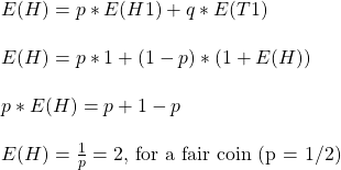
You toss a coin once: it can land on H with probability p and T with q or (1 -p). If it is H, the game ends after one flip. The value (for the time to wait) becomes 1, and the expected value, E(H), for an H start is p x 1. On the other hand, if the flip ends up with T, you start again for another flip. In other words, you did 1 flip, but back to E(H). The expected value, in this case, is (1-p)x(1 + E(H)). The final E(H) is the sum of each starting possibility.

\\ E(H) = p*E(H1) + q*E(T1)\\ \\ E(H) = p*1 + (1-p)*(1 + E(H)) \\ \\ p*E(H) = p + 1 - p \\ \\ E(H) = \frac{1}{p} = 2 \text{, for a fair coin (p = 1/2)}

This should not come as a surprise. Since p is the probability of getting heads (say, 1/2), you get an H on an average 1/p (2) flip if you flip several times.

Expected waiting times for HT

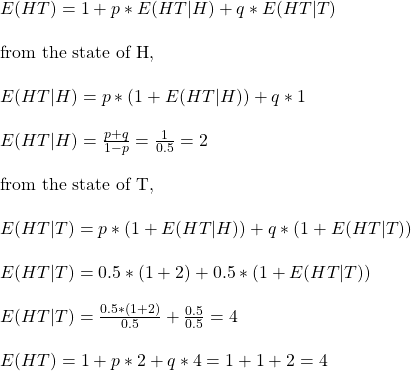
We follow the same logic again. You made one flip (1), and you have two possibilities as starting – p x E(HT|H) and q x E(HT|T). HT|H means H followed by T given H has happened. For the second flip, you either start from the state of H or from the state of T.

\\ E(HT) = 1 + p*E(HT|H) + q*E(HT|T) \\ \\ \text{from the state of H, } \\ \\ E(HT|H) = p*(1 + E(HT|H)) + q*1 \\ \\ E(HT|H) = \frac{p + q}{1 -p} = \frac{1}{0.5} = 2\\ \\ \text{from the state of T, } \\ \\ E(HT|T) = p*(1 + E(HT|H)) + q*(1 + E(HT|T)) \\ \\ E(HT|T) = 0.5*(1 + 2) + 0.5*(1 + E(HT|T)) \\ \\ E(HT|T) = \frac{0.5*(1 + 2)}{0.5} + \frac{0.5}{0.5} = 4 \\ \\ E(HT) = 1 + p*2 + q*4 = 1+1+2 = 4

Expected waiting times for HH

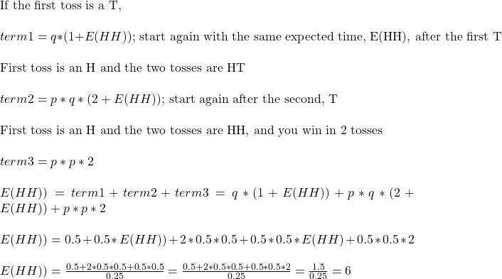
We’ll use a different method here.

\\ \text{If the first toss is a T, } \\ \\ term1 = q*(1+E(HH)) \text{; start again with the same expected time, E(HH), after the first T}\\ \\ \text{First toss is an H and the two tosses are HT } \\ \\ term2 = p*q*(2+E(HH)) \text{; start again after the second, T}\\ \\ \text{First toss is an H and the two tosses are HH, and you win in 2 tosses} \\ \\ term3 = p*p*2 \\ \\  E(HH)) = term1 + term 2+ term3 = q*(1+E(HH)) + p*q*(2+E(HH)) + p*p*2  \\ \\ E(HH)) = 0.5 + 0.5*E(HH)) + 2*0.5*0.5 + 0.5*0.5*E(HH) + 0.5*0.5*2 \\ \\ E(HH)) = \frac{0.5+2*0.5*0.5+0.5*0.5}{0.25} = \frac{0.5+2*0.5*0.5+0.5*0.5*2}{0.25} = \frac{1.5}{0.25} = 6

Waiting for Heads Read More »

Coin Flip Game

We are back to our favourite topic – coin-flipping. Anna and Ben are playing a game of flipping coins. They aim for a pattern and whoever gets it there wins. Anna chooses head-tail (HT) and Ben for head-head (HH). Who do you think will win?

You may assume since the probability of getting HT or HH in two tosses is the same, i.e., 1 in 4, the chances of winning should be identical. But the game is not about two tosses. The game is about several tosses and then counting who got the most. Let’s do this game first before getting into any theories. The following R code executes the game 10000 times, each with 5000 flips at a time, and calculates the number of times they get their respective patterns.

library(stringr)

redo <- 10000
flip <- 5000

streak <- replicate(redo, {
toss <- sample(c("H", "T"), flip, replace = TRUE, prob = c(1/2,1/2))
toss1 <- paste(toss,collapse=" ")
count <- str_count(toss1, c("H H"))

})

mean(streak)


streak <- replicate(redo, {
toss <- sample(c("H", "T"), flip, replace = TRUE, prob = c(1/2,1/2))
toss1 <- paste(toss,collapse=" ")
count <- str_count(toss1, c("H T"))

})

mean(streak)

The answer I got was 833.17 for Ben (HH) and 1249.76 for Anna (HT). Divide the number of flips with these numbers, and you get the average waiting times for the pattern. They are 5000/833.17 = 6 and 5000/1249.76 = 4. So, on average, Anna needs to wait for four flips, and Ben needs six before getting the pattern.

Pattern of three

Let us extend this for 3-coin games. Using the following code, we find the average waiting time for the three patterns – HHT, HTH, and HHH.

```{r}
library(stringr)

redo <- 10000
flip <- 5000

streak <- replicate(redo, {
toss <- sample(c("H", "T"), flip, replace = TRUE, prob = c(1/2,1/2))
toss1 <- paste(toss,collapse=" ")
count <- str_count(toss1, c("H H T"))
})

flip/mean(streak)


streak <- replicate(redo, {
toss <- sample(c("H", "T"), flip, replace = TRUE, prob = c(1/2,1/2))
toss1 <- paste(toss,collapse=" ")
count <- str_count(toss1, c("H T H"))
})

flip/mean(streak)

streak <- replicate(redo, {
toss <- sample(c("H", "T"), flip, replace = TRUE, prob = c(1/2,1/2))
toss1 <- paste(toss,collapse=" ")
count <- str_count(toss1, c("H H H"))
})

flip/mean(streak)

The waiting times are 8, 10 and 14 flips, respectively, for HHT, HTH and HHH.

Chances not identical

We will look at the theoretical treatment in another post. But first, let us try and understand it qualitatively. While the probability of getting both those two-coin sequences (or three in the second game) may be the same, the game they played takes different pathways depending on each outcome.

Look at the game from Anna’s point of view (she needs HT to win): Imagine she starts with H. The next can be an H or a T. If it is a T, she wins. But if she gets an H, she doesn’t win, but a win is just a toss away, as there is a 50% chance for her to get a T in the next flip. In other words, her failure gives her a headstart for the next.

On the other hand, Ben also starts with an H. Another head, he wins, but a tail, he needs to start all over again. He must get an H and aim for another H. A 25% chance of that happening after a failure.

Coin Flip Game Read More »