Data & Statistics

Self Biases

We shall see two interesting cognitive bises today – related to self! They are self-assessment bias and self-serving bias. From the psychological perspective, they both originate from our want to uphold self-worth and protect our ego.

Self-assessment bias, also known as the Dunning–Kruger effect, makes people overestimate their abilities. A famous example is a survey in the 80s at General Electric. The average engineer rated her performance inside the 78th percentile, and only two of the 92 surveyed thought they were below average!

On the other hand, self-serving bias is the tendency of the individual to claim credits if things go right (and blame others when wrong). While it may have originated from our desire to build and maintain high self-esteem, in the end, the results appear miserable and seriously impede our chances to learn from mistakes and succeed in life.
Self Biases Read More »

Linda’s Troubles

We have discussed the conjunction fallacy in Linda’s problem. While there are no two opinions on the notion that it is a fallacy, let’s explore why this is so normal to people. Before that, what is Linda’s problem? It is a common fallacy when people fall into the trap of selecting rare events which fit their existing stereotypes among options that include more probability. For example, people are happy to conclude that Linda is a banker and feminist versus just a banker once they hear the description that she is single, a fighter for social justice, etc.

More information supports arguments. Mathematically, AND between two statements signifies a joint occurrence, which is smaller (or equal at the maximum) than the smallest of probabilities. But it is perfectly normal for real humans to add more details and facts if we want to prove something. So, when they see multiple statements separated by an AND, they get a feeling for the validity of the statement. And if one of the statements fits their pre-existing notion, it becomes even more convincing.

Linda’s Troubles Read More »

Losses and Real Player

The issue with Thaler’s results is in the experiments themselves. Hypothetical questions answered by students are about to produce perfect answers! Real decision-makers, however, may behave differently.

First, there is no real money involved in those games. True decision-makers, accountable for gains and losses of real money, are only a minority of the population who might respond to such experimental questions. Therefore the sample may not even represent the right crowd.

Losses and Real Player Read More »

Losses and Rational thinker

In an earlier post, we have seen Thaler’s observations on how prior outcomes (wins or losses) impact the behaviour of a decision-maker. Thaler designed experiments to understand such behaviours using Kahneman and Tversky’s prospect theory. His hypotheses are called editing rules, which suggest that people edit outcomes in the way that makes them happiest.

Further to the experimental results that we have seen before, Thaler went on to do more that led to modifications of the editing rules to quasi-hedonic editing rules. Let’s see what he found.

Segregate gains, integrate losses

Results of the first experiment made the impression that people like to spread gains (happiness). The opposite, integration of the losses, although hypothesised, was not observed always. For example, in the second question of the previous post, Mr A, who lost $100 and $50 in two separate instances, is more up-happy than Mr B, who lost $150 once.

Response of a rational thinker to losses

Following is an interesting, albeit perfect, set of answers from university students.

1) Lose $9 vs Lose $9 after having lost $30. Loss of $9 hurts more in: Most of the subjects chose the second option.
2) Lose $9 vs Lose $9 after having lost $250. Loss of $9 hurts more in: There was almost 50:50 for either.

You may be wondering if this is how things happen to real people. It could be true for people who are answering the question without having to lose anything! It could also be true for people who lose money from factors which were not entirely their fault. But what about players, such as gamblers? Well, that is for another time.

Richard Thaler and Eric Johnson, “Gambling with the House Money and Trying to Break Even: The Effects of Prior Outcomes on Risky Choice”, Management Science, 1990.

Losses and Rational thinker Read More »

Skewness and Kurtosis

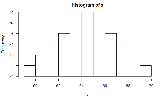
Skewness is the measure of symmetry or the lack of it. A symmetric dataset means data is distributed equally on the left and right of the mean (or median). Following is an example of a symmetric distribution.

Skewness

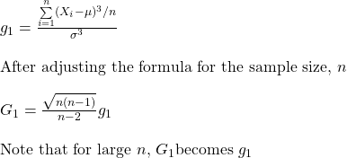
It is defined as (Pearson’s moment coefficient of skewness)

g_1 =  \frac{\sum\limits_{i = 1}^n(X_i - \mu)^3 / n}{\sigma^3} \\ \\ \text{After adjusting the formula for the sample size, }n \\ \\ G_1 = \frac{\sqrt{n(n-1)}}{n-2} g_1 \\ \\ \text{Note that for large } n \text{, } G_1 \text{becomes } g_1

The skewness of the data is close to zero for symmetric distribution, which is the case with the figure above. A positive value for g1 indicates positive skewness or right-tailed, and a negative g1 is for negative skewness or left-tailed.

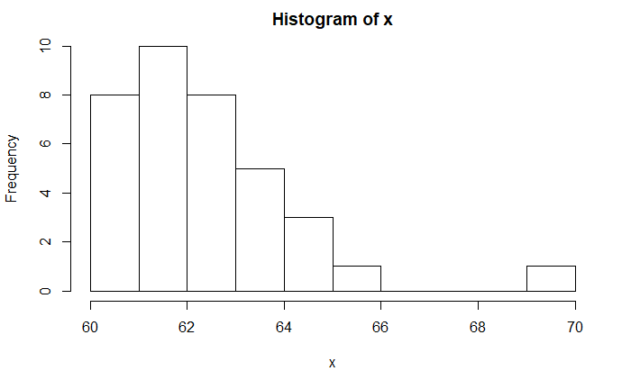
Following is an example of a positively skewed distribution (right-tailed). Its skewness is calculated to be 1.08 using the R function, ‘skewness’ (you must install library ‘moments‘ for that).

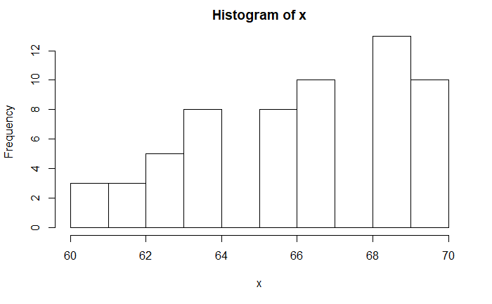
In the same way, the skewness of the following plot is -0.43; it is a negatively skewed distribution (left-tailed).

Kurtosis

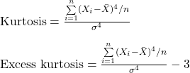
Kurtosis is the measure of how heavy or light the tail is.

\\ \text{Kurtosis}  =  \frac{\sum\limits_{i = 1}^n(X_i - \bar{X})^4 / n}{\sigma^4} \\ \\ \text{Excess kurtosis}  =  \frac{\sum\limits_{i = 1}^n(X_i - \bar{X})^4 / n}{\sigma^4} - 3\\ \\

A kurtosis value of 3 indicates standard normal distribution. Excess Kurtosis (Kurtosis – 3) is a deviation from a standard normal distribution.

Finally, the codes used to generate those distributions and their properties.

library(moments)


x <- c(rep(59.99999, each = 1), rep(61, each = 2), rep(62, each = 3), rep(63, each = 4), rep(64, each = 5), rep(65, each = 6), rep(66, each = 5), rep(67, each = 4), rep(68, each = 3), rep(69, each = 2), rep(70, each = 1))
hist(x, breaks = 10)

skewness(x)
kurtosis(x)

x <- c(rep(60, each = 8), rep(62, each = 10), rep(63, each = 8), rep(64, each = 5), rep(65, each = 3), rep(66, each = 1), rep(70, each = 1))
hist(x, breaks = 10)

skewness(x)
kurtosis(x)

x <- c(rep(60, each = 1), rep(61, each = 2), rep(62, each = 3), rep(63, each = 5), rep(64, each = 8),
rep(66, each = 8), rep(67, each = 10), rep(69, each = 13), rep(70, 10))

hist(x, breaks = 10)
skewness(x)
kurtosis(x)

Skewness and Kurtosis Read More »

What Monty Must Do

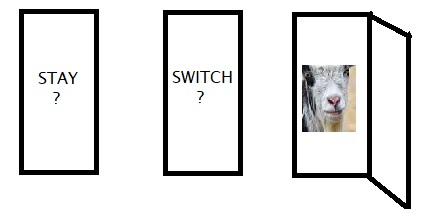
This one is about what Mr Monty shouldn’t do in the game show! The discussion on the “ideal” Monty Hall problem is available in a different post. Nonetheless, a quick proof is here. Suppose the player chose door 1 and Monty opened door 2, the probability of the car behind door 1 given Monty opened door 2 is P(C1|D2). Applying the Bayes’ formula,

\\ P(C1|D2) = \frac{P(D2|C1)*P(C1)}{P(D2|C1)*P(C1) + P(D2|C2)*P(C2) + P(D2|C3)*P(C3)} \\ \\ P(C1|D2) = \frac{(1/2)*(1/3)}{(1/2)*(1/3) + 0*(1/3) + (1*(1/3))} = \frac{1}{3} \\ \\ P(C3|D2) = 1 - 0  -  P(C1|D2)  = \frac{2}{3}

Explanation

The prior probabilities, P(C1), P(C3) and P(C3), are all equal at 1/3. P(D2|C1) = 1/2 because Monty can not open D1, and only D2 or D3 (one out of two) is available. P(D2|C2) = 0 since Monty can never open D2 if the car is behind the door 2. Since the car really exists behind one of those doors, P(C1) + P(C3) + P(C3) and P(C1|D2) + P(C2|D2) + P(C3|D2) are both unity.

The real-life Monty vs the perfect problem

The motivation for this post is when I read somewhere that Monty Hall did not always open the door in the game show. If that was true, then the TV show presented a different uncertainty than what should’ve been a calculated risk due to probability.

What Monty Must Do Read More »

Basics Continued

Continuing from the previous post, we will calculate a few more properties. We start with percentiles.

2152944506173
3163244516274
9193244526975
12203745546979
12223848546988
15263849567290
15283850577293

Percentiles

Percentile, Px, is the value below which x percentage of the data lies. It is calculated as:

P_x \approx \frac{x(n+1)}{100}

For the problem described above, P10 = 10 x 50 / 100 = 5, for n = 49. I have marked the fifth element of the table in bold (12). Similarly, P90 = 90 x 50 / 100 = 45. The 45th element is 75.

quantile(machine, 0.1)
quantile(machine, 0.9)

Quartiles

Extending it further, we can get the quartiles as P25 (first quartile, Q1), P50 (second quartile, or median, Q2), and P75 (third quartile, Q3). P25 comes out to be (25 x 50 /100), the 12.5th element. You either round it off to the nearest whole number (13) and select the 13th number, which is 26 or take the 12th number and add 0.5x(13th – 12th) = 22 + 0.5 x (26 – 22) = 24. Or 25% of the instruments will fail by 24 weeks. Similarly, P75 = 37.5th element = 69.

Inter-Quartile distance (IQD) is the difference between Q1 and Q3. Here, 69 – 26 = 43.

Variance

Variance is the measure of the variability of the data from the mean

\text{population variance } = \frac{\sum\limits_{i = 1}^n(X_i - \mu)^2}{n}

The square root of the variance is the well-known standard deviation.

\sigma = \sqrt{\frac{\sum\limits_{i = 1}^n(X_i - \mu)^2}{n}}

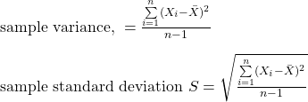
Note that the above equations are for the population. The corresponding entities for the sample are

\\  \text{sample variance, }  = \frac{\sum\limits_{i = 1}^n(X_i - \bar{X})^2}{n -1} \\ \\ \text{sample standard deviation }S = \sqrt{\frac{\sum\limits_{i = 1}^n(X_i - \bar{X})^2}{n -1}}

Chebyshev’s theorem

It is an empirical rule to predict the proportion of observations likely to lie between an interval defined using mean and standard deviation.

P(\mu - k\sigma \le X \le \mu + k\sigma) \ge 1 - \frac{1}{k^2}

For example, what proportion of data lies between two standard deviations? It is 1 – 1/22 = 0.75 or 75%. In our case, the mean is 44.94, and the standard deviation is 24.19. The interval is between [44.94 – 2 x 24.19] and [44.94 + 2x 24.19] or between -3.44 and 93.32. The number of data between these is everything or 100%! So Chebyshev gives an approximation lower than the exact. You may recall that for normally distributed data, two standard deviations cover about 95% of the data.

Basics Continued Read More »

Back to basics

We have seen and used them before. But let’s refresh a few basic statistical parameters once again. The mean time between failures (MTBF) of an instrument (in weeks) is as per the following table. Calculate the key parameters to summarise the performance.

2232442905620
3932932281238
75693761543879
15451215624950
88744438695751
15691648447252
7226919735450

There are 49 data points in total. We will estimate the mean, median, mode, and time for 10% (P10) and 90% (P90) to fail.

Central Tendency

Mean, median and mode give the central tendency of the data. The mean is the average of the data. Sum all the numbers and divide by the total number (49).

\text{Mean } = \bar{X} = \frac{\sum\limits_{i=1}^{n}X_i}{n} = \frac{2202}{49} = 44.94

#The R code is
machine <- c(22, 32, 44, 2, 90, 56, 20, 3, 93, 29, 32, 28, 12, 38, 75, 69, 37, 61, 54, 38, 79, 15, 45, 12, 15, 62, 49, 50, 88, 74, 44, 38, 69, 57, 51, 15, 69, 16, 48, 44, 72, 52, 72, 26, 9, 19, 73, 54, 50)
mean(machine)

The median represents the mid-value of the data, i.e. 50% of the observations are below the median, and 50% are above. Let us rewrite the table in ascending order. The median is the value at the position (n+1)/2 if n is odd, and if n is even, it is the average between (n/2)th and (n+2)/2th. Since the number of observations is 49 (odd), the median is the 25th element, 45, which is highlighted in bold.

2152944506173
3163244516274
9193244526975
12203745546979
12223848546988
15263849567290
15283850577293
median(machine)

Mode is the most frequently occurring value(s) in the set. In our case, 15, 38, 44 and 69 occur the maximum (3 times). Since there is no in-built function for mode in R, we create one.

stat_mode <- function(x) {
  ux <- unique(x)
  tab <- tabulate(match(x, ux))
  ux[tab == max(tab)]
}
stat_mode(machine)

Back to basics Read More »

Randomness and Clustering

We have seen the birthday problem more than once. It was initially a difficult proposition to accept that it takes only 40 people to have a match of birthdays (with 90% probability). That comes from a misconception about randomness. You have assumed that randomness meant things must spread out equally. In other words, there should be close to 365 people for two people sharing a birthday. In random processes, clustering is so natural, whereas non-clustering requires effort.

Think about an experiment in which 365 boxes lie in a line. And balls are falling from the sky. What is the probability that these balls will fill equally in each box? It is so hard for the falling balls to distribute equally without aggregation. And the reason? It’s random, and there is no brain behind the fall!

Randomness and Clustering Read More »

House Money Effect

We have already seen decision making based on expected value and utility functions (of gains and losses). The typical stories consider isolated affairs, but real life is full of connected events. The real question is how and whether prior losses and gains influence the behaviour of the decision-maker.

In gambling, it has been found that prior gains can increase willingness to gamble more (house money effect), and previous losses do the opposite. It is on that premise that Thaler and Johnson conducted experiments and asked the participants the following questions.

  1. Mr A was given two lotteries. He won $50 in one and $25 in another. Mr B was given one lottery and won $75. Who was happier? 64% of the subjects thought A was happier.
  2. Mr A received a letter from the tax authorities that he made a mistake in the returns and was required to pay $100. He received another note on the same day for another $50. Mr B got one letter from the authorities for $150. Who was more upset? 75% of the participants thought it was A.
  3. Mr A’s car was damaged in a parking lot and had to spend $200 on repairs. The same day he won a lottery for $25. Mr B’s car was damaged and he had to spend $175. Who was more upset? 70% answered B.
  4. Mr A won a lottery for $100, but on the same day, he damaged the rug in his apartment and had to pay $80 to his landlord. Mr B bought a lottery and won $20. Who was happier? An overwhelming majority thought it was B.

Richard Thaler and Eric Johnson, “Gambling with the House Money and Trying to Break Even: The Effects of Prior Outcomes on Risky Choice”, Management Science, 1990.

House Money Effect Read More »