Data & Statistics

Gambler’s Trouble Continues

We will continue the gambler’s trouble; through probability and binomial trials. The probability of making exactly one dollar after playing three even-money bets (payoff 1 to 1) of an American Roulette is given by the following binomial relationship:

nCs x ps x q(n-s) = 3C2 x (18/38)2 x (20/38)(3-2)

What we did here was to calculate the chance of winning two games and losing one (out of three) to win one dollar. But that is not a reasonable estimate. What is more realistic is to estimate the probability of winning at least one dollar in three games.

3C2 x (18/38)2 x (20/38)(3-2) + 3C3 x (18/38)3 x (20/38)(3-3)

Another way of estimating the same is to use the cumulative density function (CDF). In R, we know how to estimate it.

sim_p = 18/38
1 - pbinom(1, 3, prob = sim_p)

pbinom function calculates the total probability starting from the smallest value of zero winning. pbinom(1, 3) is the cumulative probability density of up to win, i.e., chance of zero wins out of three + one win out of three. But what we require is: at least two wins, which is (1 minus up to 1 win). By the way, it is 0.46 (46%).

In the same way, what is the probability of making at least one dollar profit if you bet 100 games at one dollar each?

sim_p = 18/38
1 - pbinom(50, 100, prob = sim_p)

The answer is about 27%. If you go for 1000 games, the probability falls to 4.5%. Play for 10000, and you will never win a dollar (p = 0.00000006567867)

Gambler’s Trouble Continues Read More »
The Depth of Gambler’s Troubles

Roulette stories are back. We will generate thousands of games with R programming utilising the probability of winning in a typical Roulette game. The sample function in R can produce random output at the specified probability values. For example,

sim_p <- (18/38)
sim_q <- 1 - sim_p
sample(c(1,-1), size = 1, prob = c(sim_p, sim_q), replace = TRUE)

The above code will generate payoffs for even-money bets (odd/even, red/black) using the probabilities for success = (18/38) and failure = (20/38). If you win, you get $1; else, you lose $1. If you play more than one, provide that number at the size option.

Now, we will use the replicate function to generate hundreds of copies of the same calculation, simulating the scenario of several players gambling and will estimate various statistics. For simulating 1000 players,

B <- 1000
gamble <- replicate(B, {
gamble <- sum(sample(c(1,-1), size =1, prob = c(sim_p, sim_q), replace = TRUE))
})

The code gives the total amount that each of the 1000 players gets. Now, put the whole calculations in a for-loop and estimate the money each player gets by playing up to 10000 games. Then evaluate two statistics: the average amount of total money a player could get and the number of players who made money (> $0) in the betting.

sim_p <- (18/38)
sim_q <- 1 - sim_p

game_x <- 10000

game_nu <- seq(1:game_x)
win_nu <- seq(1:game_x)
win_mon <- seq(1:game_x)

for (game in 1:game_x){
  
     B <- 1000
     win_amt<- replicate(B, {
            amount <- sum(sample(c(1,-1), size = game, prob = c(sim_p, sim_q), replace = TRUE))
     })

     game_nu[game] <- game
     win_mon[game] <- mean(win_amt)
     win_nu[game] <- sum(win_amt > 0) 
}

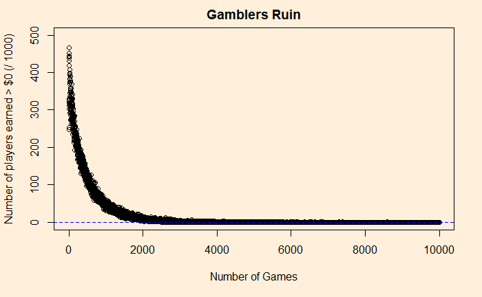
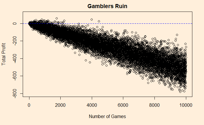
The out gives three vectors – game_nu, win_mon, and win_nu for, respectively, game number, total money gained and the number of people (out of 1000) who won at least a dollar in the end. The plots are below.

Graph 1
Graph 2

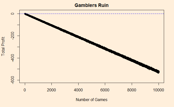
Note that the first graph represented the average loss, which averaged over 1000 players. And that is the reason why it appears as a neat, straight line. In reality, it will be a scatter like the following.

Graph 3

Yes, a few players can still make a dollar after playing 2000-3000 games (as seen in graph 2). Beyond that, not even a single player makes anything positive.

The Depth of Gambler’s Troubles Read More »

Detox and Cleansers

The significance of detox is not just about spreading myths or exploiting human phobias; it’s also about the multi-billion dollar industry that thrives on our ignorance. But before we examine why it is pointless to try and clean your body by consuming something or doing some breathing exercise, let us first understand why ideas that flush out stuff from the body are sold so readily.

Easy to relate

It is easy to visualise accumulated dirt and the attack of enemies. If you have blocked drainage, you send liquid cleaners down. If the enemy attacks, send soldiers and smoke them out. It is a fallacy called the false analogy. Another one is the appeal to (common) belief. So, when your trusted traditional healer asks you to drink plenty of water and then vomit them out, you feel assured and feel happy after spitting out the bitter (must be the bad stuff in the body!) liquid.

Your real cleaner

Part of the reason we readily buy the plumbing argument is our lack of knowledge about our bodies. The liver is a vital organ in our body that, among scores of other things, is the gatekeeper against harmful substances. It breaks down the food we consume and sends the good stuff to the bloodstream and the waste to the kidneys.

Now, think about what happens when you drink your favourite detox drink, which contains a couple of vegetables, perhaps a lemon and a few herbs. It gets digested, nutrients are absorbed in the blood, and they reach the liver. Alas, not knowing this was a cleaner meant to clean it up, the liver breaks them down and packs any valuable things, e.g. vitamins, into the body and the waste to the kidneys.

What can you do for your cleaner?

The least you can do is not to overwhelm it. Avoiding the overconsumption of alcohol tops the list. Get vaccinated against Hepatitis (B and C), the viral infection that affects the liver. Finally, be careful with detox agents, especially the overload of unknown natural stuff, which often damages your liver or kidneys.

Read

Detoxing body: The Guardian

The water myth: McGill

Detox deception: The nature education

Body stuff with Dr Jen Gunter: TED

4 detox myths: MD Anderson

Detox and Cleansers Read More »

The Weight of Energy Transition

Global warming concerns everybody because it triggers climate change or the long-term change in the average weather patterns.

Not a small problem

The world needed 600 EJ (ExaJoules of energy) in 2019. So what is an ExaJoule? It is an energy unit, which equals 1018 Joules (1 followed by 18 zeros). To put it in perspective, the energy consumed by your 10 W LED bulb in one hour is 36000 Joules. Another unit to describe energy is TWh (terawatt hour). 600 EJ is approximately 167,000 TWh.

So, what is the issue with this energy? Out of this 600, 490 are directly connected to CO2 emissions. Or that energy is produced by burning fuels containing carbon atoms in it – you call it coal, crude oil or natural gas. Let’s look at the split in the year 2019.

OilCoalNatural
Gas
BiofuelsNuclearHydroWind
Solar
18716214057301513

The Weight of Energy Transition Read More »

Origins of the Black Death

We have been seeing some marvellous acts of bio-detectives in recent years. In yet another monumental feat of locating the proverbial needle in the haystack, scientists of the Eberhard Karls University of Tübingen have unearthed the origins of the bubonic plague of the mid-14th century.

In a paper published yesterday in the prestigious journal Nature, Spyrou et al. describe how DNA sequences of samples from seven individuals exhumed from two of the cemeteries in Kara-Djigach and Burana of the modern-day Kyrgistan.

The team collected the tooth samples from Peter the Great Museum of Anthropology and Ethnography in St Petersburg. The specimens were excavated between 1885 and 1892. The tombstone inscriptions suggest that the victims were dead between 1338 and 1339. DNA extractions were done from the tooth powder using standard extraction reagents, and voila: they see DNA sections of Yersinia pestis (Y. pestis), the bacterium responsible for killing about 60% of the population of western Eurasia!

What is more? The study identified the DNA as the common ancestor to the bacteria strains that ran havoc in central Eurasia.

The source of the Black Death in fourteenth-century central Eurasia: Nature

Origins of the Black Death Read More »

Paired t-Test

The final episode of this series is a paired t-test. We have done it before, manually. Today we will do it using R.

The exercise we did earlier was on a weight-loss program. “Company X claims its weight-loss drug success by showing the following data. You’ll test whether there’s any statistical evidence for the claim (at a 5% significance level)“.

BeforeAfter
120114
9495
8680
111116
9993
7883
7874
9691
132136
108109
9490
8891
101100
9390
121120
115110
102103
9493
82 81
8480

The null hypothesis, H0: (weight before – after) = 0.
The alternative hypothesis, HA: (weight before – after) > 0.

We insert the data in the following command and run the function, t.test.

A_B_data <- data.frame(Before = c(120, 94, 86, 111, 99, 78, 78, 96, 132, 108, 94, 88, 101, 93, 121, 115, 102, 94, 82, 84), After = c(114, 95, 80, 116, 93, 83, 74, 91, 136, 109, 90, 91, 100, 90, 120, 110, 103, 93, 81, 80))

t.test(A_B_data$Before, A_B_data$After, paired = TRUE, alternative = "greater")

Note that we went for a one-tailed (right side) test as we wanted to verify the increase (the option, alternative = “greater”), not just a change from the reference value.

Paired t-test

data:  A_B_data$Before and A_B_data$After
t = 1.6303, df = 19, p-value = 0.05975
alternative hypothesis: true difference in means is greater than 0
95 percent confidence interval:
 -0.08179912         Inf
sample estimates:
mean of the differences 
                   1.35 

There was a difference of 1.35, yet the p-value was higher than the critical value we chose (0.05). The test shows no evidence to prove its effectiveness. Therefore, the null hypothesis is not rejected.

What was the significance level?

A few questions remain, did we choose a significance level of 0.05 or something else? We think we used 0.05, but we chose only one side of the t-distribution. That will partially mean a far higher tolerance level (0.05 instead of 0.025 in a two-tailed). So, what is the right way? These are valid questions, and we will answer them in a future post.

Paired t-Test Read More »

2-Sample t-Test

The purpose of the two-sample t-test is to compare the means of two groups and determine whether any difference exists between the two.

Here, we evaluate the difference between two schools following two different teaching methods, using their assessment scores. The null and alternative hypotheses are:

N0 = the means for the two populations are equal.
NA = The means of the two populations are not equal.

Method AMethod B
60.12 70.62
65.773.7
70.182.1
62.1472.14
71.877.1
62.163.1
64.9 80.4
64.8 61.3
59.160.1
65.9 75.8
66.8 78.5
61.5 69.9
58.2 70
61.8 82.1
65.979.1

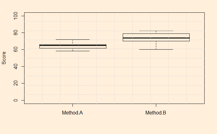
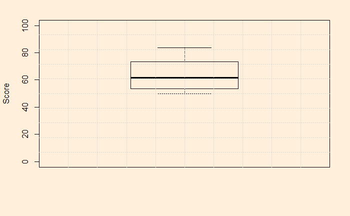
As done before, we plot the data first; we use a box plot.

2-Sample t-test

The R code for the 2-sample t-test is the same (“t.test”) as before, but you need to input both sets of data in it.

AB_data <- data.frame(Method.A = c(60.12, 65.7, 70.1, 62.14, 71.8, 62.1, 64.9, 64.8, 59.1, 65.9, 66.8, 61.5, 58.2, 61.8, 65.9), Method.B = c(70.62, 73.7, 82.1, 72.14, 77.1, 63.1, 80.4, 61.3, 60.1, 75.8, 78.5, 69.9, 70, 82.1, 79.1))

t.test(AB_data$Method.A, AB_data$Method.B, var.equal = TRUE)
	Two Sample t-test

data:  AB_data$Method.A and AB_data$Method.B
t = -4.2402, df = 28, p-value = 0.00022
alternative hypothesis: true difference in means is not equal to 0
95 percent confidence interval:
 -13.357755  -4.655578
sample estimates:
mean of x mean of y 
 64.05733  73.06400 

Before jumping to the answers, you may have noticed that I have used var.equal = TRUE here. In other words, I have assumed the variances of each group to be equal; well, more or less similar! Depending on the variances, there are two methods: the standard method is used when the variances are similar. When they are different, we need to use the Welch t-test. Let’s check the standard deviations of the groups. They are 3.86 and 7.27.

We’ll make no assumptions here, and I repeat the calculations using var.equal = FALSE. Here are the results.

t.test(AB_data$Method.A, AB_data$Method.B, var.equal = FALSE)

	Welch Two Sample t-test

data:  AB_data$Method.A and AB_data$Method.B
t = -4.2402, df = 21.308, p-value = 0.0003561
alternative hypothesis: true difference in means is not equal to 0
95 percent confidence interval:
 -13.42015  -4.59318
sample estimates:
mean of x mean of y 
 64.05733  73.06400 

Similar answers suggest that variances are, indeed, close to each other.

Interpreting results

We will start with the p-value now. p = 0.0003561, which is less than the standard significance level of 0.05. Therefore, we can reject the null hypothesis. i.e., the sample data suggest that the population means are different.

The 90% confidence interval [-13.4, -4.6] escapes zero, which is no more a surprise and reinforces the fact that the null hypothesis, zero difference between the means, is not valid here. The negative sign on the difference only means that the mean of method A is lower than method B.

2-Sample t-Test Read More »

Interpreting t-Test Results

In the previous post, we have done a 1-sample t-test on students’ scores to check for statistically significant changes from the past year’s average. Today we will spend time interpreting the results. First, the results:

	One Sample t-test

data:  test_data$score
t = 1.9807, df = 19, p-value = 0.06229
alternative hypothesis: true mean is not equal to 50
95 percent confidence interval:
 49.80912 56.92088
sample estimates:
mean of x 
   53.365 

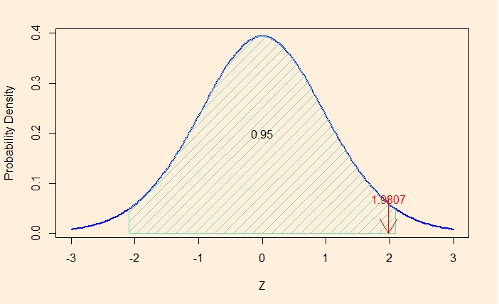
Since there were 20 data points in the study, the degree of freedom (df) is 19. The sample mean is 53.365, which is higher than the reference value of 50; however, the calculated t-value is 1.9807. If you choose alpha (the significance level) to be 0.05 (5%), the t-value should be more than 2.09 to reject the null hypothesis. In other words, 1.9807 is within the 95% confidence area (of the t-distribution).

Remember that not being able to reject the null hypothesis doesn’t mean that you accept the null hypothesis. In simple terms, there is no way to say that the population mean for this year remained at 50. The 95% confidence interval tells you that the actual population mean is between 49.80912 and 56.92088, i.e., the range includes the reference value (50).

Of course, it also doesn’t mean that the sample mean of 53.365 is the new population mean!

Finally, the dear old p-value: the p-value is more than 0.05, which is the standard significance level we chose in the analysis. It is 0.06229.

Interpreting t-Test Results Read More »

1-Sample t-Test

We will do a 1-sample t-test from start to finish using R. You know about the t-test, and we have done it before.

What is a 1-sample t-test?

It is a statistical way of comparing the mean of a sample dataset with a reference value of the population. The reference value (reference mean) becomes the null hypothesis and what we do in the t-test is nothing but hypothesis testing.

Assumptions

There are a few key assumptions that we make before applying the test. First, it has to be a random sample. In other words, it has to be representative; otherwise, it would not provide any valid inference for the population. The second condition requires that the data must be continuous. Finally, the data should follow a normal distribution or have more than 20 observations.

Example

You have done a major revamp of the school curriculum this year. You know the state-level average test score last year was 50. You like to find out whether the average score this year is different from the previous. So, you conducted a random sample of 20 participants, and their scores are below:

StudentScore
140.5
250.1
360.2
451.3
542.1
657.2
737.9
847.2
958.3
1060
1161.2
1252.5
1366
1455
1558
1655.1
1747.4
1852.1
1963.1
2052.1
mean = 53.365

Is that significant?

The mean = 53.365 suggests there was an improvement in students’ scores. But that is a quick conclusion; after all, we took only a sample, which will have variability, and, unlike the population mean, the sample means will follow a distribution. So we will do testing the following hypotheses:

The null hypothesis, N0: The mean of the population this year is 50
The alternative hypothesis, NA: The mean of the population this year is not 50
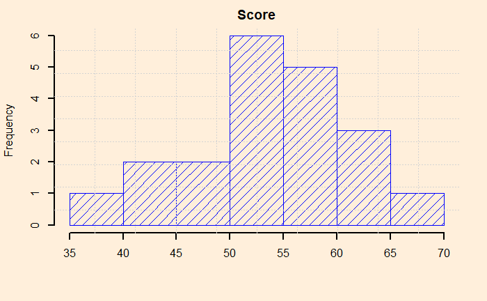
But, before that, let’s plot the data. It is a good habit that can already give a feel of the data quality, scatter, outliers etc.

The data look pretty ok, with no outliers, reasonably distributed etc. Now, the t-test. It’s simple: use the R function, t.test (stats package), and you get everything.

test_data <- data.frame(score = c(40.5,50.1,60.2, 51.3, 42.1, 57.2, 37.9, 47.2, 58.3, 60, 61.2, 52.5, 66, 55, 58, 55.1, 47.4, 52.1, 63.1, 52.1))
t.test(test_data$score, mu = 50)

The output is as follows

	One Sample t-test

data:  test_data$score
t = 1.9807, df = 19, p-value = 0.06229
alternative hypothesis: true mean is not equal to 50
95 percent confidence interval:
 49.80912 56.92088
sample estimates:
mean of x 
   53.365 

We shall see the inferences of this analysis in the next post.

1-Sample t-Test Read More »

Ecological Fallacy – What Radelet Saw

Michael Radelet’s study in 1981 is an example of ecological fallacy but, more importantly, exposed the racial disparity that existed in the process of ensuring criminal justice in the US.

Radelet collected data from 20 counties of Florida indictments of murders that occurred in 1976 and 1977. His research team have identified 788 homicide cases, and after cleanup of incomplete information, 637 remained for further investigation.

Ecology

Let us start with the overall results: the race composition of the death penalty is 5.1% (17 death penalties out of a total of 335 defendants) for blacks and 7.3% (22 out of 302). There is nothing much in it, or if you are right-leaning with a bit of vested interest, you might even say the judges are more likely to hand death penalties to the whites!

The details

Now, what happens to justice if the victims were white? If the person died in the case was white, there is a 16.7% chance for the black defendants to get a death sentence vs 7.7% for a white. On the other hand, if the person murdered was back, the percentages are 2.2 for blacks and 0 for whites. Black lives were priced lower, and whites seemed to have some birth rights to take out some of it!

The complete dataset is below; you may do the math yourself.

# CasesFirst degree
indictments
Sentenced
to Death
Non-Primary
White victim
Black defendant635811
White defendant15112419
Non-Primary
Black victim
Black defendant103566
White defendant940
Primary
White victim
Black defendant310
White defendant134733
Primary
Black victim
Black defendant166510
White defendant840
Total63737139

Radelet, M.L.; Racial Characteristics and the Imposition of the Death Penalty, American Sociological Review, 1981, 46 (6), 918-927

Ecological Fallacy – What Radelet Saw Read More »