Data & Statistics

Sum of Dice

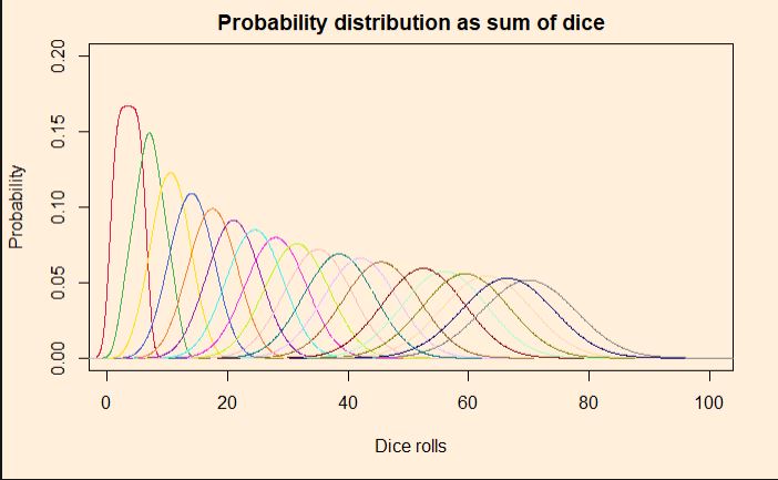
We have seen how outcomes from games with uniform probabilities add up to a normal distribution. Today we make a little R program that simulates this and plots the probability densities on one graph. In the end, we will explore how to construct the normal distribution that it approximates. Here is the plot that shows the rolling of up to 20 dice, starting from a single one.
Simulating the dice

As usual, we use the sample() function to throw out random outcomes by providing six options with equal probabilities. The sampling is then placed inside a loop that keeps on adding outputs.

plots <- 20
sides <- 6
   roll_ini <- replicate(100,0)
   roll <- sample(seq(1:sides), 1000000, replace = TRUE, prob = replicate(sides,1/sides))
   Dist_ini <- density(roll, bw=0.9)
 
   par(bg = "antiquewhite1")
   plot(Dist_ini, ylim=c(0,0.2), xlim=c(1,100), main="Probability distribution as sum of dice", xlab = "Dice rolls", ylab =  "Probability")

 for (i in 1:plots){
   roll <- roll_ini + sample(seq(1:sides), 1000000, replace = TRUE, prob = replicate(sides,1/sides))
   Dist <- density(roll, bw=0.9)
   mycolors <- c('#e6194b', '#3cb44b', '#ffe119', '#4363d8', '#f58231', '#911eb4', '#46f0f0', '#f032e6', '#bcf60c', '#fabebe',  '#008080', '#e6beff', '#9a6324', '#fffac8', '#800000', '#aaffc3', '#808000', '#ffd8b1', '#000075', '#808080', '#ffffff', '#000000')
   lines(Dist, col = mycolors[i])
   roll_ini <- roll
 }

We then derive the normal distribution that corresponds to the above. The mean and standard deviation of rolling a die are:

\\ \text{ mean } = E[X] = \sum\limits_{i=1}^6 x_i p_i = x_1p_1 + x_2p_2 + x_3p_3 + x_4p_4 + x_5p_5 + x_6p_6 \\ \\ = 1 * \frac{1}{6} + 2 * \frac{1}{6} +3 * \frac{1}{6} +4 * \frac{1}{6} +5 * \frac{1}{6} +6 * \frac{1}{6} = \frac{21}{6} = \frac{7}{2}  = 3.5\\\\ \text {for n rolls,} \\ \\ E[X_1 + X_2 + ... + X_n] = E[X_1] + E[X_2] + ... + E[X_n] \\ \\ E[X + X + ... + X] = E[nX] = nE[X] = 3.5*n \\ \\  \text{variance} = Var[X] = E[(X - \mu)^2] \\ \\ Var[X]  = \sum\limits_{i=1}^6 \frac{1}{6}  (i-\frac{7}{2})^2) = \frac{1}{6} [ (- \frac{5}{2})^2 + (- \frac{3}{2})^2 + (- \frac{1}{2})^2 + (\frac{1}{2})^2 + ( \frac{3}{2})^2 + ( \frac{5}{2})^2] \\ \\ Var[X] = \frac{35}{12} \\ \\ \text{standard deviation } = \sigma = \sqrt{(Var[X])} =  \sqrt{\frac{35}{12}} \\ \\  \text {for n rolls,} \\ \\ Var[(X+Y)] = Var[X] + Var[Y] + Cov(X,Y) \\ \\ Var[(nX)] = n*Var[X] + 0 \text{ , } Cov(X,X) = 0\\ \\ Var[(nX)] =  \frac{35}{12} n \\\\ \sigma =  \sqrt{\frac{35}{12} n}

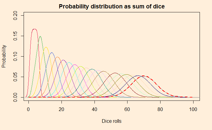
Add the following line at the end, and you get the comparison for normal distribution for rolls of 20 dice summed over.

norm_die <- 20
lines(seq(0,100), dnorm(seq(0,100), mean = norm_die*(7/2), sd = sqrt(norm_die*(35/12))), col = "red",lty= 2, lwd=2)
Sum of Dice Read More »

Sum of Uniform Distributions

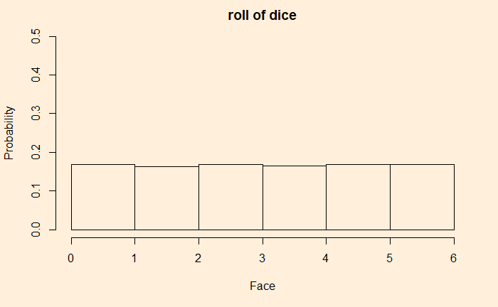
You know what happens if you roll a fair die; you get one of the six faces. But what happens when you try it 10000 times and plot the frequency or the probability?

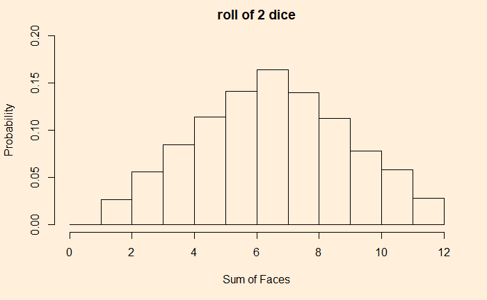
We have a uniform distribution with probability = 1/6. What happens if we throw two dice and plot the distribution of their sums?

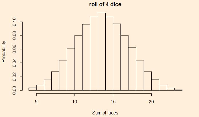
It resembles a triangular distribution with a maximum probability of getting seven as the sum. Let’s not stop here: add the outcomes of four dice.

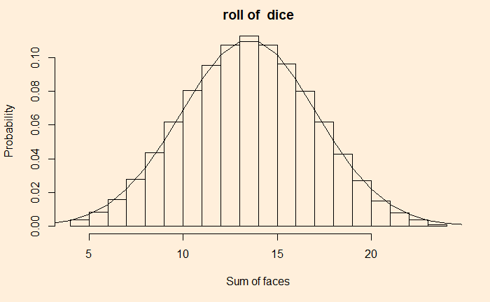
It appears more like a uniform distribution. Let’s insert one such distribution and see how it looks.

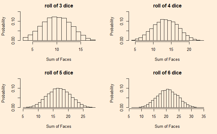
We can see the more the number of such random outcomes we add (more number of dice together), we approach the realm of the central limit theorem.

Sum of Uniform Distributions Read More »

Estimating Poker Hands

Let’s calculate a few poker probabilities for the 5-card hands. We employ basic calculations and some simulations.

5 hands from 52 cards

First, what is the total number of ways of getting five cards from a deck of 52? Is that a permutation or a combination? The fundamental question to ask is whether the order matters or not. The order of cards doesn’t matter here; hence we use combinations to get the required value.

_{52}C_5 = \frac{52!}{(52-5)!5!} = \frac{52!}{47!5!} =  2,598,956

Royal flush

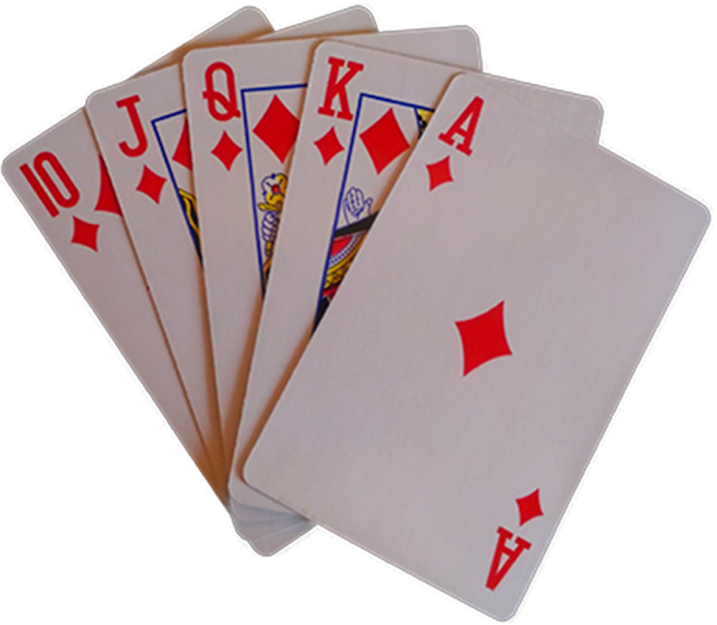
This one comes first in the order and has a sequence of 10, J, Q, K, A, of a given suit.

poker, casino, games-2015890.jpg

The calculation is simple: Getting this combination out of five cards is 5C5 = 1. Since there are four types (suits), clubs, diamonds, spades and hearts, the total number becomes 4. The required probability of getting a royal flush is (4/2,598,956) = 0.00000154. Let’s do the simulation

First, create the deck

suits <- c("Diamonds", "Spades", "Hearts", "Clubs")
numbers <- c("Ace", "Deuce", "Three", "Four", "Five", "Six", "Seven", "Eight", "Nine", "Ten", "Jack", "Queen", "King")
deck <- expand.grid(Number = numbers, Suit = suits)
deck <- paste(deck$Number, deck$Suit)

Then we write the following code to simulate the chances of getting a royal flush.

roy <- c("Ace", "Ten", "Jack", "Queen", "King")
royal <- expand.grid(Roy = roy, Suit = suits)
royal <- paste(royal$Roy, royal$Suit)

itr <- 10000000

poker <- replicate(itr,{
   shuffle <- sample(deck, 5)
      for (rep_trial in 1:4) {
          if(all(shuffle %in% royal[(5*rep_trial-4):(5*rep_trial)])==TRUE){
             counter <- 1
             break
          }else{
             counter = 0
         }
      }
     counter <- counter
})
mean(poker)

After running 10 million times, we get 12 occurrences and therefore, the probability is 0.0000012

Estimating Poker Hands Read More »

Areas through Monte Carlo

You may have known how to evaluate a definite integral or integrals bounded within limits. For example, consider the following:

\int_0^1 x^2 dx

We can estimate the value by integrating the function y = x2 and applying the limits.

\int_0^1 x^2 dx = \frac{x^3}{3}|_0^1 = \frac{1}{3}

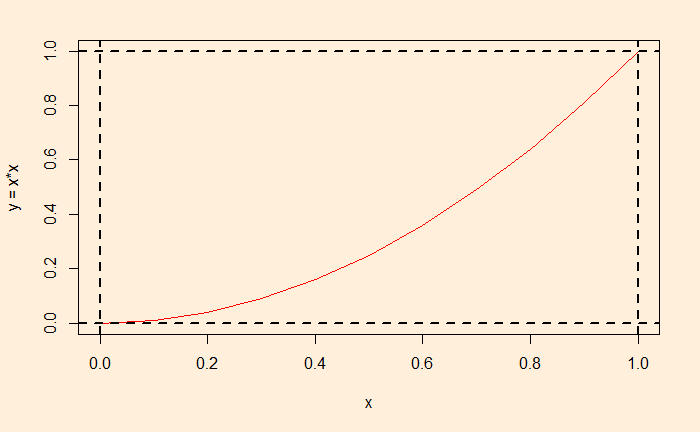
The function (within those bounds) is plotted below, and the required integral is the area under the curve.

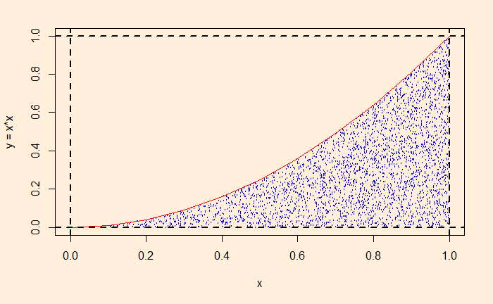
Looking at the graph above, one can envision that the required area is the fraction of a unit square at which the relationship, y </= x2 works. As we have done before, we will fill the unit square by selecting random numbers between 0 and 1 and collect the fraction that obeys the equation. This this:

itr <- 10000

xxx <- replicate(itr,0)
yyy <- replicate(itr,0)
counter <- 0

for (rep_trial in 1:itr) {
  
  xx <- runif(1)
  yy <- runif(1)
  if(yy <= xx*xx){
    xxx[rep_trial] <- xx
    yyy[rep_trial] <- yy
    counter <- counter + 1
  }
}
counter/itr

And the output (the integral, counter/itr) is 0.3312.

Simulations like these, the probability of hitting between the restricted boundaries of a unit square, are handy for estimating areas under functions that are difficult to integrate analytically.

Areas through Monte Carlo Read More »

The Probability of A Flat Tyre

At Duke University, two students had received A’s in chemistry all semester. But on the night before the final exam, they were partying in another state and didn’t get back to Duke until it was over. Their excuse to the professor was that they had a flat tire, and they asked if they could take a make-up test. The professor agreed, wrote out a test and sent the two to separate rooms to take it. The first question (on one side of the paper) was worth 5 points, and they answered it easily. Then they flipped the paper over and found the second question, worth 95 points: ‘Which tire was it?’

Source: Marilyn vos Savant, Parade Magazine, 3 March 1996, p 14.

The question for today is: What is the probability for the students to get the second question right?
1) If the students have no preferences for a specific tyre?
2) If they have the following preference: right front, 58%, left front, 11%, right rear, 18%, left rear, 13%?

Counting

Let’s address the first problem by counting all possibilities.

RFLFRRLR
RFRF,RFRF,LFRF,RRRF,LR
LFLF,RFLF,LFLF,RRLF,LR
RRRR,RFRR,LFRR,RRRR,LR
LRLR,RFLR,LFLR,RRLR,LR

There are a total of 16 possibilities, and four of them (highlighted in bold) are common. So the required probability for two students having the same random answers is 4/16 or 1/4.

Adding joint probabilities

Another way to reach the answer is by adding the joint probabilities of each of the four guesses. P(RF, RF) + P(LF, LF) + P(RR, RR) + P(LR, LR). P(RF, RF) is the joint probability of both the students arriving at the right front independently. If each one has a (1/4) chance, P(RF, RF) = P(RF) x P(RF) = (1/4)(1/4) = (1/16). Collecting all of them, P = P(RF) x P(RF) + P(LF) x P(LF) + P(RR) x P(RR) + P(LR) x P(LR) = (1/4)(1/4) + (1/4)(1/4) + (1/4)(1/4) + (1/4)*(1/4) = (1/4).

For the second question: P = 0.58 x 0.58 + 0.11 x 0.11 + 0.18 x 0.18 + 0.13 x 0.13 = 0.3978 or about 40%.

Simulation

Let’s run the following R code and verify the answer.

iter <- 10000
lie_count <- replicate(iter, {
   studentA <- sample(c(1,2,3,4), size = 1, replace = TRUE, prob = c(0.25, 0.25, 0.25, 0.25))
   studentB <- sample(c(1,2,3,4), size = 1, replace = TRUE, prob = c(0.25, 0.25, 0.25, 0.25))

   if(studentA == studentB){
     counter = 1
   }else{
     counter = 0
  }
})
mean(lie_count)

Output: 0.2532.

Change the probabilities, and you get the second one:

iter <- 10000
lie_count <- replicate(iter, {
   studentA <- sample(c(1,2,3,4), size = 1, replace = TRUE, prob = c(0.58, 0.11, 0.18, 0.13))
   studentB <- sample(c(1,2,3,4), size = 1, replace = TRUE, prob = c(0.58, 0.11, 0.18, 0.13))

   if(studentA == studentB){
      counter = 1
   }else{
      counter = 0
   }
})
mean(lie_count)

Output: 0.3971.

The Probability of A Flat Tyre Read More »

Odds and Probabilities

You must have heard of the odds of winning bets. It says what kind of bet you would be willing to make. It is often confusing as there are several conventions to describe. We will see them one by one and understand the associated probabilities.

Odds in stats

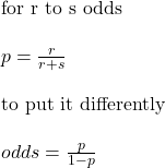
A 2 to 1 odds means that out of three possible outcomes, there will be 2 of one kind and 1 of another. It means there is a probability of 2/3 (66.7%) for one and 1/3 (33.3%) for the other. The relationship is:

\text{for r to s odds} \\ \\ p = \frac{r}{r+s} \\ \\ \text{to put it differently} \\ \\ odds = \frac{p}{1-p}

For p = 2/3, odds = (2/3)/(1-(2/3)) = 2/3/1/3 = 2/1.

The odds of rolling a six in a die is 1 to 5. This means one outcome will favour a six, and five do not.

In gambling

Things take a slightly different turn in gambling. The odds in gambling focus on winning the stake and, therefore, represent the amount the bookmaker pays along with the original bet. Odds of 4/1 means the bettor stands to make 4 profit on a stake of 1 (gets a total of 4 + 1 = 5). And there are four styles of betting odds:

1. Americal style

Boston Celtics: +450
Golden State Warriors: +550
Milwaukee Bucks: +800

Those mean: If you bet 100 on the Celtics, you win 450; a total payout of 550. Warriors: bet 100, win 550, payout of 650. Finally, the bucks can win you 800 and a payout of 900 for a 100 bet.

Odds with a negative sign in front mean how much money you need to bet to win 100. So -200 means you get 100 if you bet 200 (total payout = 100 + 200 = 300).

2. Decimal style

Multiply the decimal with the wager, and you get the payout. So for the Celtics case, the decimal odd is 5.5. Bet 100, and you get 5.5 x 100 = 550 as the payoff.

3. Fractional style (UK)

Like the American style, this calculates the profit and not the payout. a/b (a-to-b) means your profit is (a/b) x wagered amount. So for the Celtics, the fractional odds are 4.5/1 or 9/2.

4. Implied odds

It is the probability equivalent in the betting world. A 9-to-2 odds imply it is an underdog with a chance of 2 out of 11 for winning or 18.18%.

Sports betting odds: The Sports Geek

Odds and Probabilities Read More »

Random Walker Continued

Follow the profit

The R function that fits well with this objective is cumsum(). For example, here is what it gives if you apply it to the vector (1, 4, 2, 3, 6):

cumsum(c(1, 4, 2, 3, 6))  # gives

#   1  5  7 10 16

It sums as it goes along: 1, 1+4=5, 5+2=7, 7+3=10, 10+6=16

Let’s use it on a set of 10,000 random outcomes of a coin. For that, we need to generate random numbers with the correct values for the profit and loss at 50:50 probabilities. Then plot the outcome.

n <- 10000
xx_f <- sample(c(-1, 1), n, TRUE, prob = c(1/2, 1/2))
x_val <- cumsum(xx_f)
plot(x_val, type = "l", col = "blue", ylim = c(-150,100), xlab = "", ylab = "")

Don’t assume that this is the only outcome you can expect. If I run the same program four more times, here is what you get:

So, anything is possible! But not all equally likely, as can be seen below:

Your intuition is correct; the maximum probability of occurrence for the H is 5000, which means the profit is zero. Again, not to forget: the absolute probability of getting 5000 may be the highest, about 80 out of 10000, yet that is not what you see in real life because not getting zero overwhelms (10000 – 80)! You can also see that chances of getting a gain of 200 (5100 Hs) or a loss of 200 (4900 Hs) are still possible, but with a lower likelihood. But, a gain (or a loss) of 400 is really rare.

Gambler’s ruin

While any of the above plots may be used to illustrate a gambler’s ruin, we will use our favourite roulette wheel; probability 18/38 for a win and 20/38 for a loss. The random walk is dramatic here for a 10000-long run.

You can try as many times as possible; getting a positive value at the end of this walk is unlikely!

Random Walker Continued Read More »

Path of a Random Walker

Let’s demystify the concept of probability games and the law of large numbers with coin-tossing as an example.

Law of large numbers

We know what it means: when one estimates the mean of several thousand outcomes of an experiment, the result converges to the expected value or the theoretical average. For example, if one tosses a coin a million times, the mean head becomes 0.5 or 50%. Recall the plot we developed earlier.

But that is deceptive. It gives a feeling that if you play a million games, with 1$ for a head and -1$ for a tail, your wallet remains unchanged, whereas if the game is short, you gain or lose more money. That is not true.

Higher absolute, lower average

In the coin tossing game, how do you calculate the average head? It is the number of occurrences of heads divided by the number of games played. If I play only one game and get a head, it is 1, and tail, it is 0, the two extreme average values you can ever get (1/1 and 0/1). If it was a game described in the earlier section, you may gain a dollar or lose one. On the other hand, if you play 100 games and win 60, you get 20 dollars (60-40), and the mean head is 60/100 = 0.6. If you play a million games and win 184 more heads than tails, the mean is even smaller and close to the theoretical (500092/1,000,000 = 0.50009). But you gain more money ($ 184) and can also lose more money.

Random walk

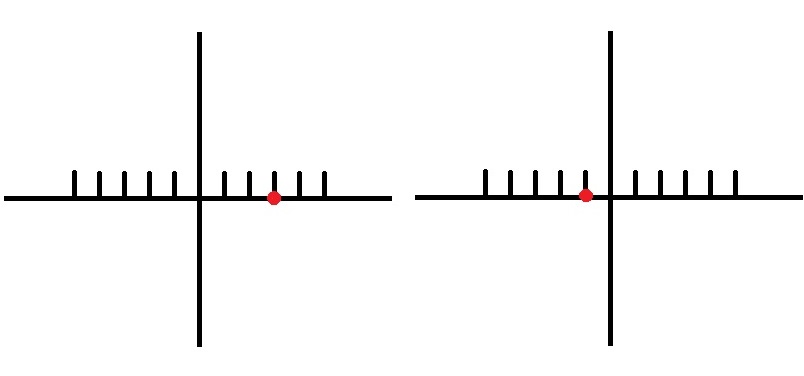
The figure we saw in the earlier section showed the average and not the absolute gain. To display the successes and flops of the games played, you resort to a random walk model. Imagine you are standing at the intersection of the X and Y axes, i.e. at zero. You play, and if you win, you move one unit to the right, and if you lose, you move one to the left.

Here are two such walks. On the left, the walker had the following outcomes: H, H, T, H, H. This is equivalent to 1, 1, -1, 1, 1 in terms of money and 1, 2, 1, 2, 3 in terms of position from the origin. The corresponding moves of the right walker are (outcome H, H, T, T, T), (money 1, 1, -1, -1, -1) and (position 1, 2, 1, 0 -1).The last digit of the position vector is the current position after five games.

To sum up

To sum up: the law of large numbers doesn’t mean if you play a large number of coin-tossing games, you win or lose nothing. It only means that the effort you put in (gain per game or the money per time) diminishes with games. The walker moves further and further from the origin, although the rate of change becomes slower. We will see more on the random walks in the next post.

Path of a Random Walker Read More »

Probabilistic Insurance

Probabilistic insurance is a concept introduced by Kahneman and Tversky in their 1979 paper on prospect theory. Here is how it works.

You want to insure a property against damage. After inspecting the premium, you find it difficult to decide to pay for the insurance or leave the property uninsured. Now, you get an offer for a different product that has the following feature:

You spend half the premium but buy probabilistic insurance. In this case, you have a probability p, e.g. 50%, in which you, in case of damage, will pay the rest of the 50% and get fully covered, or the premium is reimbursed, and the damage goes uncovered.

For example, the scheme works in the first mode (pay the reminder and full coverage) on odd days of the month and the second mode (reimbursement and no coverage) on even days!

Intuitively unattractive

When Kahneman and Tversky asked this question to the students of Standford university, an overwhelming majority (80%) was against the insurance. People found it too tricky to leave insurance to luck or chances. But in reality, most insurances are probabilistic, whether you are aware or not. The insurer always leaves certain types of damages outside their scope. The investigators proved using the expected utility theory that probabilistic insurance is more valuable than a regular one.

Tversky, A.; Kahneman, D., Econometrica, 1979, 47(2), 263

Probabilistic Insurance Read More »

The Shape of Randomness

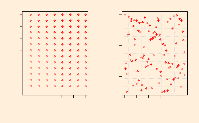
If I give a task to mark 100 random dots on a paper, which of the following two patterns do you likely to come up with?

Studies have found that there is a tendency for people to identify uniform patterns when asked about randomness. In the above picture, the one on the right was generated by a random program.

Now another: Two students were asked to toss coins 20 times and record. Following is what they came up with. If one of them made up his experiment, who could that be?

1) THTTHTTHHTTTTTHTTHTH
2) THHTTHTHTTHHTHTTHTH

Clusters in randomness

It is difficult for most people to imagine that long clusters of Ts in the first case come randomly. After all, shouldn’t the equal probabilities of occurrence of heads and tails suggest an even distribution, like in the second case?

The Shape of Randomness Read More »