Data & Statistics

Hormonal contraception and thrombosis

Studies have found that the usage of hormonal contraceptives increases the chances of thrombosis by 300 to 500 per cent. Isn’t it worrying? Definitely, it is worrying, but what is the absolute risk here?

Breaking news of the 60s

The association between certain types of oral contraceptives (that contain estrogen and progestin) with thrombosis has been known since the 1960s. Naturally, it led to attention from the media and panic in society, eventually to reduced usage and increased pregnancies.

A case of bad science reporting?

Hopefully, you have recognised the main issue with this report (remember the posts about covid vaccines and colorectal cancer.). A paper published in 2011 reviewed this case of thrombosis with root causes and relative risks. Among them was the absolute risk or the incidence of thrombosis for adults. It is 1 -10 per 100,000 per year. With the use of this type of oral contraceptive, the risk increase to 5 – 50 in 100,000 per year, which is up to 0.05%. But what about mishaps due to actual pregnancies and abortions? 

Finally, just how big is a 100% increase of a risk? Well, that depends on the absolute risk on which it is based!

Hormonal Contraception and Thrombotic Risk: A Multidisciplinary Approach: PEDIATRICS, 127(2), 2011

Hormonal contraception and thrombosis Read More »

Salamander Reporposed!

Salamanders are fascinating creatures that have drawn plenty of spotlight from biologists due to their significant position in our evolutionary path. These are amphibians, and it was no coincidence that they drew attention, as a missing piece between creatures of water and that of land, from scientists in the 19th century, inspired by the recent theory of evolution.

In one such pursuit, what the famous zoologist and the Professor at the Museum of Natural History in Paris, Auguste Dumeril, found provides a live example of the wonders of repurposing animal functions.

In 1864, Dumeril received six salamanders from a lake in Mexico. They were large adults with feathery gills and aquatic body shapes characteristic of life in water. He kept them together and even had them produce fertilised eggs. The children that came out of the cage shocked the researcher; they showed little resemblance to their parents. No gills and aquatic tail; they appeared like the terrestrial variety.

It was found out much later that there are two pathways of development for the salamander larvae, according to the surrounding environment. The salamander in the aquatic habitat goes through the default pathway, but the one on land undergoes this metamorphosis. We now know the change gets triggered by the amount of thyroid hormone in the bloodstream that activates or kills some cells. Same gene, same creature but a change of environment yielding dramatic change in the appearance of the end product!

Reference

Some assembly required: Neil Shubin

Salamander Reporposed! Read More »

Common Sense Continued

The not-so-hidden secret is that biological innovations never come about during the great transition they are associated with.

Neil Shubin, Some Assembly Required

Another case of common sense is the theory of evolution.

Theorem of evolution

While it is no more topic of debate, thanks to millions of data collected in the last one hundred odd years, the concept of evolution has confused the generations since the day it was proposed.

Evolution of common sense

The first one was the remnants of Lamarckian thinking that essentially assumes that evolution is what an organism aspires and achieves, in its lifetime, to adapt to its environment. For example, a giraffe, in pursuit of high-lying leaves, stretches its neck so much that its child gets her neck a little longer than her mother, and it continues.

The other group is less dramatic with their approach, though commonsensical. Feather occurred to birds because it enabled the birds to fly, which helped them to survive in that environment. Similarly, lungs and limbs happened just about when the water-living creatures prepared to come out to the land.

More and more pieces of evidence proved that this understanding is wrong. The features such as the lungs or the wings were part of predecessor creatures ages before they transformed into their next level. For example, fishes of all species had swim bladders that enabled them to navigate different depths in the water. As genetic studies have later found, the genes responsible for these air sacs are the same that propelled the development of lungs. In other words, when the fish’s successor came to land, it just repurposed the swim bladder for breathing.

Inventions to products

A closer analogy is the example of green hydrogen as a vector of decarbonised energy. Hydrogen production through water electrolysis using renewable electricity such as solar PV is considered a commercial-ready option for a carbon-free energy future. To anybody who followed the history of science, electrolysis is by no means a new technology.

Alkaline water electrolysis technology is more than 120 years old. It has been serving the niche market of caustic and chlorine until now.

Similar story for solar PV. Bell Labs announced a solar battery in 1954 that could produce electricity whenever a thin slice of silicon was contacted by sunlight, being celebrated as a miracle device by the leading newspapers of that time. At the time of its invention, it was so expensive that Bell Labs calculated a cost of $1.5m to power one home using their technology!

But nothing happened for another 65 years!

Repurposing under societal pressure

This chemistry of evolution, where the ingredients were made in the distant past, but mixing happens only today, has confused people and led to creating two bands of commentators. The first group, the Vaclav Smil-type, develops some allergy to “high-tech worshippers” and claims whatever happens today was a result of the 1880s. The second group are mesmerised by the speed at which discoveries are happening right in front of their eyes. Both got carried away by the chemistry of evolution.

Common Sense Continued Read More »

Climate Change and Common Sense

To all the people in the northern hemisphere who are currently reeling under extreme heat waves: your assessment of global warming is correct, but not for the reasons you think you are seeing.

Common sense is a general intelligence that enables a person to manage concrete everyday situations. It is common sense to switch the power off before removing a bulb from its holder. Wearing a protective glove before touching the metal pot on the kitchen hob is another.

In a survey conducted in Australia between 2010-14, 22% of the respondents thought climate change was not happening. When specifically asked about what their opinions are based on, about 37% of them attributed to common sense. It might sound absurd that about 20% of the people who believed in human-induced climate change also attributed their belief to common sense. And the views of both parties are not surprising. Phenomena such as global warming are understood only through the laborious examination of scientific data from hundreds of sources through the lens of mathematical models. And there is nothing commonsensical about it!

The offspring of hindsight

It is a fact that some of the lessons learned from science can later become part of the common sense knowledge in everyday life. But trusting that the opposite is also true is dangerous. We have seen multiple examples of logical fallacies previously. Availability bias is one of them. For a climate sceptic, the last year’s winter might be the guiding principle, whereas, for a climate believer, it’s the heat wave of this summer. One can prove either of these as instances of random events, even when the number of hard facts on climate change is irrefutable.

Overdependence on experience

Common sense is primarily a manifestation of personal experience; science, on the other hand, is a rational, evidence-based approach that operates through the collaborative actions of hundreds of trained minds. While individual scientists are fallible mortals with cognitive biases and beliefs, the rigour of methodology – validation and falsification – known as the scientific method, by its community elevates science from those shortcomings.

Climate Change and Common Sense Read More »

Occupancy Problem

In a village of 2000 people, what is the chance of finding a day in the year which is not the birthday of someone? How do you solve this problem? The solution to this problem makes use of the Poisson approximation for r entities trying to occupy n empty cells.

When r and n are high so that lambda = n exp (-r/n) is bounded, the probability of m empty cells becomes the Poisson distribution function, p(m; lambda).

In or case, lambda = 365 x exp(-2000/365) = 1.52. The required probability may be obtained by subtracting the chance of seeing no empty day from one.

1 – dpois(0,1.52) = 0.78 or 78%

Occupancy Problem Read More »

The curse of the VAERS: The Post Hoc Fallacy

Today we explore the difference between ‘after’ and ‘from’! Because it concerns a famous fallacy called “Post Hoc Ergo Propter Hoc“. So what does this cool-sounding Latin phrase mean? As per Wikipedia, it means: “after this, therefore because of this”. It is the interpretation that something happens after an event to something from it. Take the example of the CDC’s Vaccine Adverse Event Reporting System (VAERS).

Adverse Event Reporting System

The Centers for Disease Control and Prevention of the United States uses VAERS as a system to monitor adverse events following vaccination. The data was meant for the medical researchers to find patterns and, thereby, potential impacts of vaccines on human health. Naturally, the system gets scores of events ranging from minor health effects to deaths. And a section of the crowd interprets and propagates these events due to vaccination. So, where is the fallacy here?

What happened in 2020

The number of people who died in the US due to heart disease in 2020 is 696,962, which is about 2000 per million population. The figure is 1800 for cancer, 500 for respiratory illness and 310 for diabetes. So, roughly 4610 per million per year due to these four types of diseases.

Thought experiment

Let’s divide 20 million Americans into two hypothetical groups of 10 million each. The first group took the vaccine over one month, and the second did not. What is the expected number of people from the unvaccinated group to die of the four causes mentioned previously? About 3840. But they do not report to the VAERS.

On the other hand, imagine a similar death rate to the vaccinated group. If 10% of those 3840 people report the incident in the system, it will make 384 reports or about 4600 in the whole year.

The first case will be forgotten as fate, whereas the second will be celebrated by the media as: “vaccine kills thousands”!

References

Diseases and Conditions: CDC

Vaccine Adverse Event Reporting System (VAERS): CDC

The curse of the VAERS: The Post Hoc Fallacy Read More »

Managing Staff for Stochastic Births

Continuing with the Poisson distribution, we will work out an example today. The nursing supervisor of a busy hospital knows that, on average, 16 child-births happen in an 8-hr shift. How will she manage the wards, making sure the delivery service is optimally staffed?

Assuming delivery is dominated by natural delivery, which is stochastic, we resort to Poisson distribution to make the required calculations. Start with the extreme values.

What is the probability of having zero childbirth in a shift?

\\ P(X = s) = \frac{e^{-\lambda}\lambda^s}{s!} \\ \\ \text {For zero births, s = 0. And we know } \lambda = 16. \\\\ P(X = 0) = \frac{e^{-16}*1}{1} = 0.0000001125

This can also be obtained directly using the R, ppois(0,16). What is the probability of getting up to 7 births (0 – 7)? ppois(7,16) = 0.00999 or about 1%. Also, the supervisor now knows at 90% certainty that it would not be more than 21 as ppois(21,16) is 91%.

Reference

Biostatistics for Medical and Biomedical Practitioners, 2015, Pages 259-278: Chapter 18 – The Poisson Distribution

Managing Staff for Stochastic Births Read More »

Coin-Tossing – Distribution of Interval Arrival Times

We did establish Poisson distribution through coin tossing. Here we calculate the distance between the arrivals or the interarrival times. This is obtained by marking the indices of heads and then finding the difference between two successive heads.

First, we run 100000 simulations of coin-tossing and collect the heads (H) as successes in an array. Find out the indices of the array, which are nothing but the arrival times. The difference between the indices is the interarrival times.

n <- 100000
xx_f <- sample(c("H", "T"), n, TRUE, prob = c(1/2, 1/2))
index <- which(xx_f =="H")

length(index)
dist <- rep(0,length(index)-1)
for (i in 1:length(index)-1) {
  dist[i] <- index[i+1] - index[i]
}

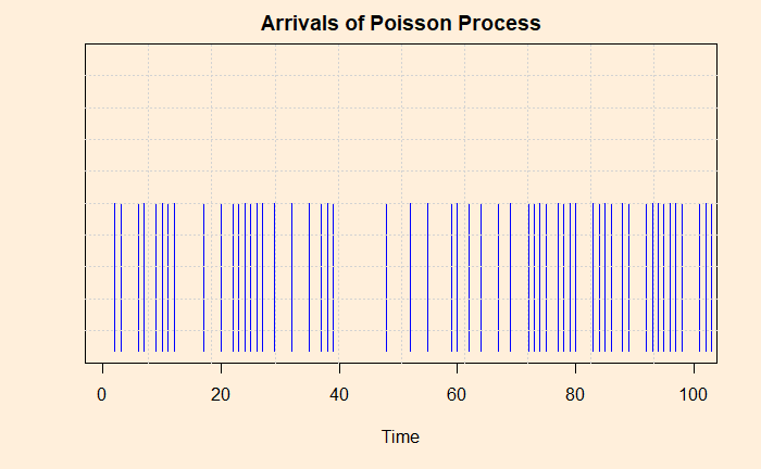
We show the first 100 appearances of H in the following plot.

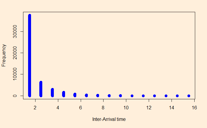
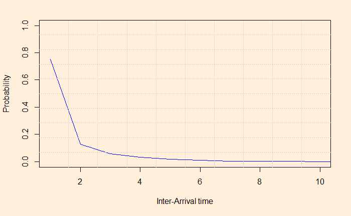
The frequencies and densities of the interval arrival distances are in the graphs.

These describe exponential distributions!

Coin-Tossing – Distribution of Interval Arrival Times Read More »

Poisson through Coin-Tossing

Coin tossing exercises are a simple but valuable means to understand a lot of real-life situations. Here we learn Poisson distribution by tossing a coin.

Poisson processes are used to model the number of occurrences of events over certain periods of time. They are discrete processes and also stochastic, i.e. the outcomes are random.

Customer arriving at a shop is often viewed as an example of the Poisson process. The shopkeeper knows the number of customers she expects in a day or an hour based on experience but never can’t predict what happens next minute. The following set of plots describes four such distributions for different mean arrivals (lambda).

As you can see, mean arrivals, coinciding with the peaks of these plots, are informative. However, the actual comings will vary between higher and lower values making certain decisions, staff allocations to support customers, for instance, very tricky.

So far, we have focussed on fixed time duration but random arrivals. You can also understand Poisson differently – a specified number of arrivals at random intervals. Look at the following graph: it describes a Poisson activity; time on the x-axis, and each vertical line denotes one appearance. Don’t waste your time on a pattern; there is no pattern!

Toss a coin

The above picture describes the tossing of a coin (e.g. every second) and marking an entry whenever a head happens.

n <- 100000
xx_f <- sample(c("H", "T"), n, TRUE, prob = c(1/2, 1/2))
index <- which(xx_f =="H")

We just plotted the index values corresponding to H.

Poisson through Coin-Tossing Read More »

Four of a Kind over Full House

Which hand is more valuable, four-of-a-kind or full-house? Well, that depends on which of the two is rarer. Let’s calculate them. If you are still unsure what I am talking about – it is about the 5-card poker game.

In a 5-card hand poker game, a player gets five cards from a well-shuffled deck of cards. Remember: one deck has 52 cards – 13 ranks in each of the four suits. The 13 ranks are 2, 3, 4, 5, 6, 7, 8, 9, 10, J, Q, K, A, and the four suits are diamonds, hearts, aces and clubs. Now, over to calculations.

The probability of a hand equals the number of ways you get a particular pattern (four-of-a-kind and full-house, in our case) divided by the total number of ways you can get five random cards from a deck of 52. If you recall some of the earlier posts, the latter is nothing but the combination, 52C5.

Four of a kind

spade, risk, chance-3081114.jpg

What is the number of possibilities to get this pattern? One way to approach this is to imagine five boxes. Your task is to fill the first four boxes with of kind (rank). There are 13C1 ways to find rank and 4C4 ways to arrange four suits from the maximum of four. So, the first four boxes can be filled by 13C1 x 4C4 number possibilities. Once the first rank is done in the first four boxes, there are 12 other ranks remaining for the last box. Using the same argument we used before, that becomes 12C1 x 4C1.

The final probability is (13C1 x 4C4 x 12C1 x 4C1) / (52C5) = 624 / 2598960 = 0.00024

Full house

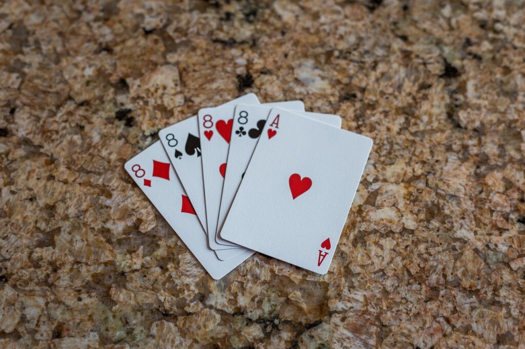
You need three of one kind and two of another to get full-house.

cards, poker, full house-6001541.jpg

Imagine the five boxes again. This time, we first fill three with 13 kinds, one at a time and four suits, three at a time. 13C1 x 4C3. The remaining two boxes need to be filled with another kind. 12C1 x 4C2. The total options are 13C1 x 4C3 x 12C1 x 4C2 = 3744 / 2598960 =0.00144.

Summary

The four-of-a-kind has a lower chance of occurrence compared to the full-house. The former is, therefore, more valuable.

Four of a Kind over Full House Read More »