Data & Statistics

Infinite Prisoner’s Dilemma

You know what a prisoner’s dilemma is. Here, each prisoner optimises the incentive (minimises the downside) by betraying the other. And the payoffs matrix is,

B CooperatesB Defects
A Cooperates(3,3)(0,5)
A defects(5,0)(1,1)

But what happens when the choices are repeated? Then it becomes an infinite prisoner’s dilemma.

Infinite game

Unlike the once-off, the player in the infinite game must think in terms of the impact of her decision in round one on the action of the other in round two etc. The new situation, therefore, fosters the language of cooperation.

Cooperation

The question is: how many games do the players need to realise the need for cooperation?

Concept of discounting

Let’s start the game. In the found round, as rational players, players A and B will play defect, leading to a mediocre, but still better than the worst possible, outcome.

Infinite Prisoner’s Dilemma Read More »
Irrationality and Stupidity

The confusion of stupidity for irrationality is common but equally a misunderstanding. While being stupid and irrational may lead to the same outcome, poor decision-making, we should realise that the two are distinctly different. Most humans are not stupids; a lot of us are irrational in something or the other.

Stupidity is the error of judgement caused by inherent limitations of intelligence. Irrationality is due to risk illiteracy or the lack of knowledge of probability. One may be mitigated; the other is doubtful.

Irrationality and Stupidity Read More »

De Méré’s Paradox

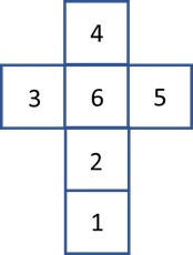
What is more probable – getting at least one six in four throws of a die or getting at least one double six in 24 throws of a pair of dice?

It is a paradox because common sense (again!) tells you that both are equally probable. The probability of getting a six for a single die is (1/6), and that for two sixes from a pair of dice is (1/6)x(1/6). So by extrapolation, what happens in four throws for a single may become six times more (24) for double dice.

Well, the answer is wrong. Here is the calculation.

One dice

One dice
A) The probability of getting a six in one roll is (1/6).
B) The probability of getting no six in a roll is, therefore, (5/6).
C) The probability of getting no sixes in four rolls is (5/6)4 = 0.48.
D) The chance of getting at least one six in four throws is 1 – 0.48 = 0.52.

A pair

Following the steps above
A) The probability of getting a double-six in a pair of rolls is (1/6)x(1/6) = 1/36.
B) The probability of getting no double-six in a pair of rolls is 35/36.
C) The probability of getting no double-six in 24 rolls of a pair of rolls is (35/36)24 = 0.51.
D) The chance of getting at least one double-sixes in 24 rolls of a pair of dice is 1 – 0.51 = 0.49.

In summary

Getting one six in four rolls is more probable than getting one double-six in twenty-four.

De Méré’s Paradox Read More »

Potato Paradox

We have seen how percentages can miscommunicate severities of diseases with low prevalences. This time we will look at another counterintuitive fact, but here, an opposite perception, showing the contrast between absolute and relative quantities – the potato paradox.

Suppose I have 100 kg of potatoes with a 99% water content. It means 99% water and 1% solids. And if I dry them to reduce their moisture content from 99 to 98%, what is the final weight of my potatoes?

Let’s perform the calculations.
Initial weight of potatoes = 100 kg
Initial water content = 99%
Initial weight of water = 99kg
Initial weight of solids = 1 kg.

Now, drying doesn’t reduce the solids.

Final weight of solids = 1 kg.
Final water content = 98%
Final solid content = 100 – 98 = 2%

If 1 kg of solids represents 2% (0.02) of a mix, the weight of the mix is 1 (kg) / 0.02 = 50 (kg). So the final weight of potatoes is 50 kg, half of the original, and the drying just managed to reduce the moisture content from 99 to 98%!

Potato Paradox Read More »

The weatherman is Always Wrong

It is easy to prove your weatherman is wrong. Easier if you are short-term memory and are oblivious to probability.

Imagine you tune into your favourite weather program; the prediction was: a 10% chance of rain today. You know what it means: almost a dry day ahead. The same advice continued for the next ten days. What is the chance there was rain on at least one of those days? The answer is not one in ten, but two in three!

You can’t get the answer by guessing or using common sense. You must know how to evaluate the binomial probability. For instance, to calculate the chance of getting at least one rain in the next ten days, you use the formula and subtract it from one.

Decision making

All these are nice, but how does this forecast affect my decision-making? The decision (take a rain cover or an umbrella) depends on the threats and alternate choices. On a day with a 10% chance of rain predicted, I will need a reason to take an umbrella, whereas, on a day of 90%, I need a stronger one not to take precautions.

Why the weatherman is wrong

Well, she is not wrong with her predictions. But the issue lies with us. Out of those tens days, we may remember only the day it rained because it contradicted her forecast of 10%. And the story will spread.

The weatherman is Always Wrong Read More »

Efron’s Impossible Dice

Here we are, with another dice dual. I hope you recall the last banana problem. The setting is the same; there are two dice to roll, and the player who gets the higher number will win. But there is a problem the dice are not the normal ones like we know.

But they are of the four following ones.

Angela and Ben are playing this game. Angela has the advantage of choosing the first die; Ben then picks from the remaining three. Which one should Angela pick? Can Angela win this game at all?

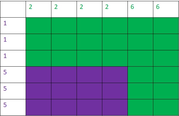
Angela thinks we can win this, for she has the first chance to choose. She compares purple and green. Let’s see what she gets. Here is the R code.

repeat_game <- 10000

win_perc_A <- replicate(repeat_game, {

   die_cast1 <- sample(c(2,2,2,2,6,6), size = 1, replace = TRUE, prob = c(1/6, 1/6, 1/6, 1/6, 1/6, 1/6))
   die_cast2 <- sample(c(1,1,1,5,5,5), size = 1, replace = TRUE, prob = c(1/6, 1/6, 1/6, 1/6, 1/6, 1/6))
     if (die_cast1 > die_cast2) {
     counter = 1
   } else {
     counter = 0
   }

}
)
mean(win_perc_A)

Well, the green wins two out of three. Here are all the possibilities in a tabular form.

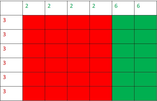
She then compares green and red, and the outcome favours red:.

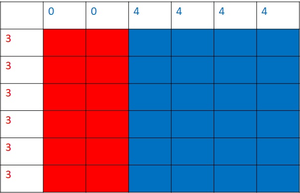
Finally, the blue and the red, and the former wins.

Since purple < green < red < blue, she thinks, blue is the winner die. And she picks it. When angela chose blue, Ben took the last one – purple. Look at the outcome.

Purple defeats blue!

Bradley Efron, professor of statistics and biomedical data science at Stanford University, is the man behind the invention of these dice. The interesting fact is that no matter which one the first person chooses, the second person always selects something better.

Efron’s Impossible Dice Read More »

Arriving at the Conditional Probabilities

We have seen the concepts of joint and conditional probabilities as mathematical expressions. Today, we discuss an approach to understanding the concepts using something familiar to us – using tables.

Tabular power

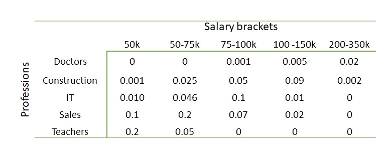
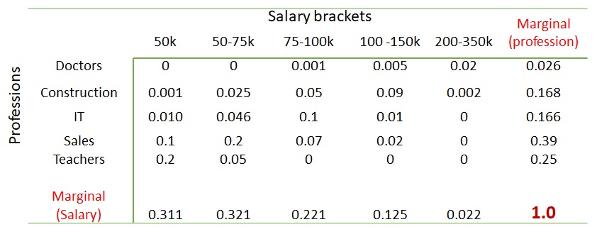
Tables are a common but powerful way of summarising data. Following is one summary from a hypothetical sample collection of salary ranges of five professionals.

It is intuitive for you to know that the values inside the table are the joint occurrences of the row attributes (professions) and column attributes (salary brackets). You get something similar to a probability once you divide these numbers by the total number of samples (= 1000). In other words, the values inside the table give us the joint probabilities.

Can you spot the marginal probabilities, say, that of doctors in that sample space? Add the numbers of the rows or columns; you get it.

Conditional probabilities

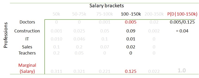
What are the chances it is a doctor if the salary bracket is 100-150k per annum? You only need to look at the column for 100-150k (because that was given) and then calculate the proportion of doctors in it. That is 0.005 out of 0.125 or 0.005/0.125 = 0.04 or 4%.

Look it this way: in the sample space, were 125 people in the given salary bracket, of which five were doctors. If the sample holds it for the population, the percentage becomes 5/125 or 4%.

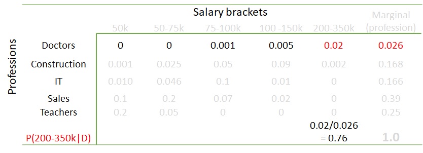
The calculation can also work in the other way. What is the probability of someone in the salary bracket of 200-350k per year, given the person is a doctor? Work out the math, and you get 76%.

Arriving at the Conditional Probabilities Read More »

Bias in a Coin – Continued

A quick recap: in the previous post, we set a target of finding the bias of a coin by flipping it and collecting data. We have assumed a prior probability for the coin bias. Then established a likelihood for a coin that showed a head on a single flip.

We know we can multiply prior with the likelihood and then divide by the probability of the data.

P(\theta|D) = P(D|\theta) * P(\theta) / P(D)

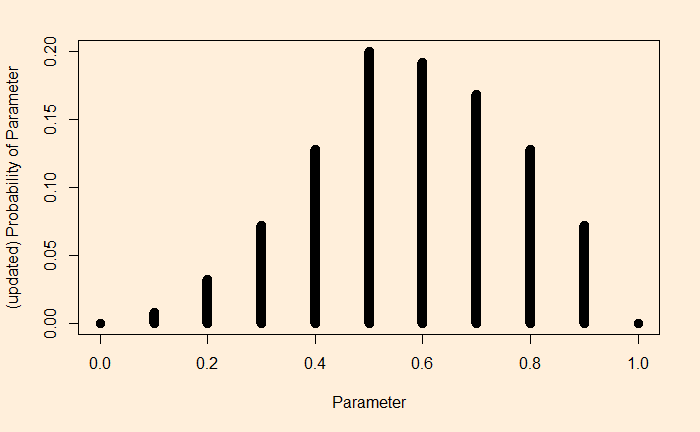
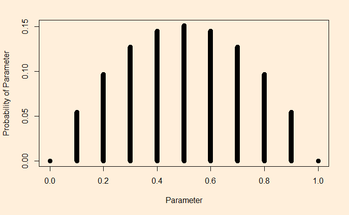
The outcome (posterior) is below.

Look at the prior and then the posterior. You see how one outcome (heads on one flip) makes a noticeable shift to the right. It is no more equally distributed to the left and the right.

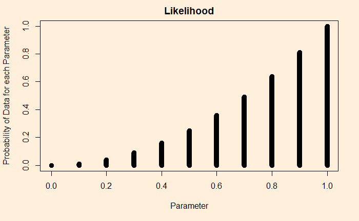
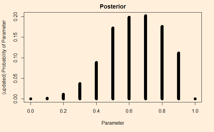
What would happen if, for the same prior, but getting two heads? First, calculate the likelihood:

You can see a clear difference here as the appearances of the two heads changed the likelihood heavily to the right. The same goes for the updated chance (the posterior).

Bias in a Coin – Continued Read More »

Bias in a Coin

Bayesian inference is a statistical technique to update the probability of a hypothesis using available data with the help of Bayes’ theorem. A long and complicated sentence! We will try to simplify this using an example – finding the bias of a coin.

Let’s first define a few terms. The bias of a coin is the chance of getting the required outcome; in our case, it’s the head. Therefore, for a fair coin, the bias = 0.5. So the objective of experiments is to toss coins and collect the outcomes (denoted by gamma). For simplicity, we give one for every head and zero for every tail.

\gamma = 1 \text{ for head and } \gamma = 0 \text{ for tail}

The next term is the parameter (theta). While the outcomes are only two – head or tail, their tendency to appear can reside on a range of parameters between zero and 1. As we have seen before, theta = 0.5 represents the state of the unbiased coin.

The objective of Bayesian inference is to estimate the parameter or the density distribution of the parameters using data and starting guesses. For example:

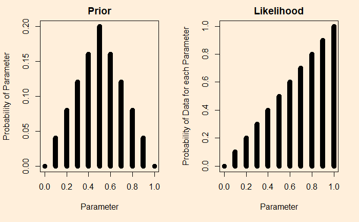
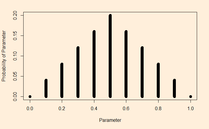
In this picture, you can see an assumed probability distribution of coins made from a factory. In a way, this is to say that the factory produces ranges of coins; we think the highest probability to be theta = 0.5, the perfect unbiased coin, although all sorts of other imperfections are possible (theta < 0.5 for tail-biased and theta > 0.5 for head-biased).

The model

It is the mathematical expression for the likelihood function for every possible parameter. For coin tosses, we know we can use the Bernoulli distribution.

P(\gamma|\theta) = \theta^\gamma (1-\theta)^{(1-\gamma)}

If you toss a number of coins, the probability of the set of outcomes becomes:

\\ P({\gamma_i}|\theta) = \Pi_i P(\gamma_i|\theta) =  \Pi_i \theta^{\gamma_i} (1-\theta)^{(1-\gamma_i)} \\ \\ = \theta^{\Sigma_i\gamma_i} (1-\theta)^{\Sigma_i(1-\gamma_i)} = \theta^{\#heads} (1-\theta)^{\#tails}

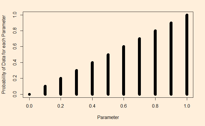
Suppose we flip a coin and get heads. We substitute gamma = 1 for each of the theta values. A plot of this function for the following type appears:

Let’s spend some time understanding this plot. The plot says: if I have a theta = 1, that is a 100% head-biased coin, the likelihood of getting a head on a coin flip is 1. If it is 0.9, then 0.9 etc., until you reach a tail-biased one at theta = 0.

Imagine, I did two flips and got a head and a tail:

The interpretation is straightforward. To take the extreme left point: If it was a tail-biased coin (the parameter, theta = 0), the probability of getting one head and one tail is extremely low. Same for the extreme right (the head-biased).

Posterior from prior and likelihood

We have prior assumptions and the data. We are ready to use Bayes’ rule to get the posterior.

Bias in a Coin Read More »

Health Screening and Some Biases

This is not a post against health screening. In fact, I did my annual checkup yesterday, something I’ve been maintaining since my 30s. Today, we critically examine a few potential challenges associated with the much-advertised benefits of cancer screening.

Survival rates

The most common metric of reporting is the survival rate. It’s the percentage population who are diagnosed with an illness that survives a particular period. Based on the local system, these periods maybe five years, ten years etc.

A long-term (2019-2013) study of prostate cancer from a French administrative entity was reported by Bellier et al. The results show the following features. The incident rate remained almost flat at around 850 per 100,000 from 1991 to 2003 for people aged 75 and over. Then the rate started decreasing at an annual rate of 7%. For the men aged 60-74, 1991 to 2005 showed a steady increase followed by a decrease similar to the older age. Overall, the younger group (60-74) had a higher 8-year survival rate (as high as 95%).

Lead time bias

Illnesses such as cancers have a particular pre-clinical phase, the time lag between the onset of disease and the appearance of symptoms. A screening test can catch the disease at this stage. The longer the pre-clinical phase, the higher the likelihood of catching early by testing. This creates a lead time in comparison with the untested. Even if the ultimate year of death is the same, the lead time adds to the statistics giving a false impression of survival rates.

Overdiagnosis

Overdiagnosis is the detection of an illness that would not have resulted in symptoms and death. As the screening rate increases, followed by treatment of the positives, it becomes difficult to know how many of them benefitted from the treatment.

Confounding

Confounding also comes to complicate the analysis. In the last few decades, along with advancements in diagnostic techniques, cancer treatments have also improved significantly, leading to higher survival chances for the early and late-diagnosed population. It makes the separation of benefits of early diagnosis less apparent.

Health Screening and Some Biases Read More »