Data & Statistics

Predicted R-Squared

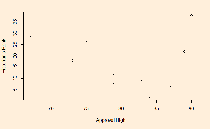
The foundation of predictive R-squared is cross-validation. We will examine the LOOCV method in this post. First, the data set that we used in the past exercises.

Approval HighHistorians Rank
2 84
687
879
983
1279
29 67
2471
2675
1068
22 89
18 73
38 90

Then,

  • The first row is removed from the list, and the regression model is developed with the other 11 data (2:12)
  • The model is used to predict observation 1 (y). By plugging in the x value (e.g. 2) in the formula (cubic form)
  • The predicted y is subtracted from the actual y for observation 1 and squared (called the squared residual)
  • Observation 1 is returned to the list, and observation 2 is removed (1, 3:12)
  • The process is continued until the last observation and squared residual are collected
  • Sum all the squared residual to get what is known as PRESS (predicted residual error sum of squares)
  • Predicted R2 = 1 – (PRESS/TSS)
res_sq <- 0
for (i in 1:12) {
  new_presi <- Presi_Data[-i,]
  model1 <- lm(new_presi$Historians.rank ~ new_presi$Approval.High +  I(new_presi$Approval.High^2) + I(new_presi$Approval.High^3))
  
  res <- Presi_Data[i,1] - (model1$coefficients[1] + model1$coefficients[2]*Presi_Data[i,2]+model1$coefficients[3]*Presi_Data[i,2]^2 +model1$coefficients[4]*Presi_Data[i,2]^3)
  
    res_sq <- res_sq + res^2
}
res_sq

The res_sq is PRESS.

TSS (or SST) is the total sum of squares = sum of (response (y) – mean of response)2

sum((Presi_Data$Historians.rank-mean(Presi_Data$Historians.rank))^2)
predict_r_sq <- 1 - (res_sq/sum((Presi_Data$Historians.rank-mean(Presi_Data$Historians.rank))^2))

Predicted R-Squared Read More »

Overfitting and Predicted R-Squared

Last time we fitted a set of data using the cubic function.

Let’s analyse the quality of the fit using the predicted R-squared method. It is also called Leave-Out-One Cross Validation (LOOCV). What it does is that it systematically leaves out one data at a time and estimates how the model performs under those circumstances. For a good fit, the predicted R-squared should be high (as close to 1).

We will estimate the predicted R-squared of the dataset using the library, “olsrr“.

library(olsrr)
model <- lm(Presi_Data$Historians.rank ~ Presi_Data$Approval.High +  I(Presi_Data$Approval.High^2) + I(Presi_Data$Approval.High^3))

ols_pred_rsq(model)

The answer is -0.2, which suggests that the cubic function is overfitting the observation.

Overfitting and Predicted R-Squared Read More »
Non-Linear Regression – Overfitting

A usual tendency in regression is to chase better R-squared by increasing the dependent variables and ending up overfitting. Overfitting is a term used when your model is too complex that it sharts fitting noise. An example is this dataset taken from Regression Analysis Book by Jim Frost. It describes the highest approval ratings of the US presidents and their rank by historians.

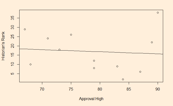
First, we try out linear regression and check the goodness of fit.

lm(Presi_Data$Historians.rank ~ Presi_Data$Approval.High)

The R-squared value is close to zero (0.006766). Now, we try cubic fit.

model <- lm(Presi_Data$Historians.rank ~ Presi_Data$Approval.High +  I(Presi_Data$Approval.High^2) + I(Presi_Data$Approval.High^3))

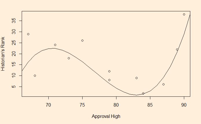
But with an impressive R-squared (0.6639)

Now, try thinking how one can explain this complex relationship, i.e. Historians Rank = -9811 + 388.9 x Approval High -5.098 x Approval High^2 + 0.02213 x Approval High^3!

Non-Linear Regression – Overfitting Read More »

Guys Finish Last

Do you remember the last time you were in a queue that reached the counter ahead of others who joined at similar times as you did? It could be a bit of a struggle to recollect, but I’m sure you remember the time you finished the last! Let’s analyse what must be happening with you.

Clue 1: Selective memory

The simplest explanation for your troubles is selective memory. Don’t you remember that day you wanted to write down a number in a phone call and found the pen was not working? You know it was not the first telephone you attended in life where you had to write something down. And you had a pen that worked, but you took it for granted – after all, the purpose of that device is to write.

You are more likely to recollect the days you finished last than you did first. And that is human nature. Biologists speculate this is part of an evolutionary defence mechanism that you remember the past incidents that led you to trouble, perhaps as a trigger not to repeat them.

Clue 2: Probability

We have seen several examples already. You are entering a billing section of a store that has ten lines. If you pick a random queue, what is the probability that you end up in the fastest? The answer is 1/10. To state it differently, what is the chance that you are not the fastest? Nine out of ten. Then you argue that it was not accidental and that you selected the shortest. There are two possible responses to that feeling.

First, all the others in the hall also (think they) selected the shortest, and your selection, regardless of how you felt, was still random. The second explanation concerns the specific information about your choice that you lacked and the others had. It was short as there was something in that queue – a slower attendant or people with items that required more time for the check-in. And you just took that. Once you are in the line and start measuring the average time taken by the others, you get into what is known as the inspection paradox.

Clue 3: WAITING-TIME PARADOX

We have seen it before in the name of the inspection paradox and waiting time paradox. We proved mathematically that the actual waiting time is longer than the theoretical average calculated based on the frequency of occurrences.

In short

Next time the feeling occurs on why it happened only to you and not anyone else, think again. It is more likely that the others, too, feel the same; after all, the “you” I chose in the description is just an arbitrary choice.

Reference

The formula for choosing the fastest queue: The conversation

Guys Finish Last Read More »

Football’s Double Poisson

It is world cup season. The world championship for football, or soccer to some, arguably one of the world’s most popular sports spectacles, is happening now in Qatar. On the eve of the start, the prestigious science journal, Nature, published an article on the importance of data science to football’s evolution to its current state.

At the end of the paper, the authors quote a prediction table based on a double Poisson model that predicted the 2020 European championship with reasonable accuracy.

Here, we “cherry-pick” one of the teams, Belgium, which failed to qualify for the knock-out stages, nonetheless the top-billed squad by the model and estimate the possibility of them qualifying from the preliminary stages.

The model estimate Belgium to have 13.88% of winning the cup, followed by Brazil at 13.51. So, we estimate that if Belgium reached the tournament’s final, it would have a 13.88/(13.88+13.51) = 50.7% chance of winning. Therefore,

The chance of winning the cup = probability of reaching the final (P1/2) x probability of winning the final.
P1/2 = 0.1388 / 0.507 = 0.27 (27%).

Extending the argument further, P1/4, the probability of Belgium in the semi-finals is, P1/4 = 0.27/(13.88/(13.88+11.52)) = 0.5.
P1/8 = 0.5/(13.88/(13.88+5.29))= 0.69.
P1/16 = 0.69/(13.88/(13.88+0.69)) = 0.72.

So, Belgium had a 28% chance of not qualifying for the playoffs, and it happened that way! Note that the chances, 11.52, 5.29 and 0.69, are taken from the same table as the winning chances of the 4th, 8th and 15th teams.

Making it broader

Here we have assumed that Belgium met Brazil (winning probability = 13.51), Argentina in the second (11.52%) etc. In reality, we don’t need to make such assumptions. Let’s consider an extreme case, which is also not possible as the qualifying teams go via a narrow path forward, where any team in the top 15 could meet Belgium in each round. We run a Monte Carlo with the following code.

nn <- 10000
  
sec_round <- replicate(nn, {
 round <- sample(c(0.1351, 0.1211, 0.1152, 0.0965, 0.0724, 0.0637, 0.0529, 0.0378, 0.0336, 0.0317, 0.0256, 0.0233, 0.0146, 0.0067), 4, replace = FALSE)

P_1 <- 0.1388
P_12 <- P_1/(P_1/(P_1+round[1]))

P_14 <- P_12/(P_1/(P_1+round[2]))

P_18 <- P_14/(P_1/(P_1+round[3]))

P_116 <- P_18/(P_1/(P_1+round[4]))

1 - P_116 
})

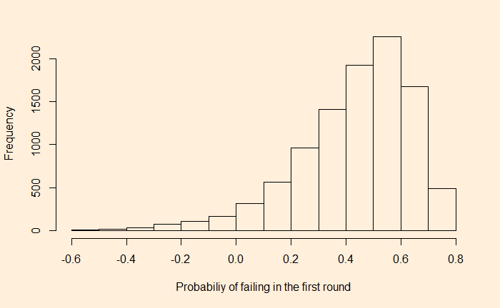
And the answer is in the following histogram.

I must say that the analysis is meant for fun, with hardly any speck of reality in it. Since the calculations are done in reverse, the conclusions don’t prove that a team with the highest (13.88%) chance to win the cup will go out from the first round with a 40% probability. On the contrary, it only states that even a team with only a 60% chance to reach the second round can still have a 13.88% chance to win!

Reference

How big data is transforming football: Nature
Double Poisson model for predicting football results: Plos One

Football’s Double Poisson Read More »

It’s All About the Fourth Quarter

Let’s turn our attention to NBA. This time, we will analyse a common belief – that the matches are decided in the fourth quarter. Apart from that, we will also try a bunch of other hypotheses, such as home-away advantage. We have collected the first 100 matches of the NBA season 2021-22 to test the hypothesis.

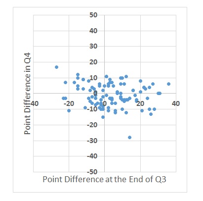
First, we check if there is any relationship between the point difference in the fourth quarter with what is at the end of the third.

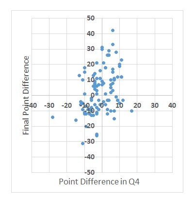
The graph shows no real relationship. So, the fourth quarter is different; but do they determine the winner? That’s next.

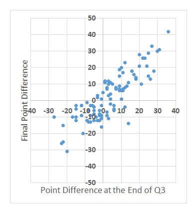
The correlation here also is modest. That brings us to the all-important graph – the winner vs the point difference at the end of the third quarter.

Winner till Q3 wins the match

The result is obvious. There seems a much better correlation between the leader until the third quarter to the ultimate winner.

It’s All About the Fourth Quarter Read More »

Probability of Rain

It’s been a while, so let’s do a probability problem. I found this one in the youtube channel “MindYourDecisions“. If it rains on a day, the probability of rain tomorrow increases by 10%; if not, it reduces by 10% for the next day. What is the probability that it will rain forever within a few days if the chance to rain today is 60%?

Let Px be the chance of raining forever, starting from a day x% rain. We can write the following equations. Note that P100 means it will rain today and every day from there. On the other hand, P0 suggest no rain today and, as a result, it continues.

P1001
P900.9P100 + 0.1P80
P800.8P90 + 0.2P70
P700.7P80 + 0.3P60
P600.6P70 + 0.4P50
P500.5P60 + 0.5P40
P400.4P50 + 0.6P30
P300.3P40 + 0.7P20
P200.2P30 + 0.8P10
P100.1P20 + 0.9P0
P00

Substituting the end value (P0 = 0) for the term P10 and working upwards,

P1001
P900.9P100 + 0.1P800.998P100
P800.8P90 + 0.2P700.98P90
P700.7P80 + 0.3P600.93P80
P600.6P70 + 0.4P500.82P70
P500.5P60 + 0.5P400.67P60
P400.4P50 + 0.6P300.51P50
P300.3P40 + 0.7P200.35P40
P200.2P30 + 0.8P100.22P30
P100.1P20 + 0.9P00.1P20
P00

The value of the last term, 0.998P100 can be evaluated by substituting P100 = 1. Repeating the exercise, now downwards,

P1001
P900.9P100 + 0.1P800.998P1000.998
P800.8P90 + 0.2P700.98P900.98
P700.7P80 + 0.3P600.93P800.91
P600.6P70 + 0.4P500.82P700.75
P500.5P60 + 0.5P400.67P600.55
P400.4P50 + 0.6P300.51P500.34
P300.3P40 + 0.7P200.35P400.18
P200.2P30 + 0.8P100.22P300.08
P100.1P20 + 0.9P00.1P200.02
P00

Therefore, the required probability is 75%.

Probability of Rain Read More »

Non-Linear Regression

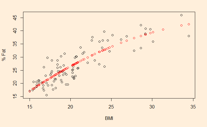
We have seen linear regression last time. While fitting a line could be a good start, one needs to exercise care before choosing it as the default. For example, see the plot below.

It gives the relationship between body mass index and body fat percentage, taken from Regression Analysis Book by Jim Frost. Warning: I’m not sure if the data was simulated or data.

Check what happens if you try and fit a straight line!


fit<-lm(BMI_Data$X.Fat ~ poly(BMI_Data$BMI,2,raw=TRUE))
quadratic = fit$coefficient[3]*BMI_Data$BMI^2 + fit$coefficient[2]*BMI_Data$BMI + fit$coefficient[1]

lines(BMI_Data$BMI,fit$coefficient[3]*BMI_Data$BMI^2 + fit$coefficient[2]*BMI_Data$BMI + fit$coefficient[1], col="red", type = "p")

Non-Linear Regression Read More »

Regression: The OLS Way

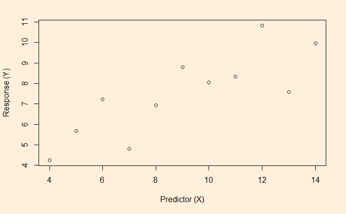
OLS is the short form for ordinary least squares and is a linear regression method. The process is also known as curve fitting informally. The objective is to find the relationship between the dependent (the y) and independent (the x) variables; one eventually gets (to predict) the variation of y from the variation of x. In case you forgot, here is the scatter plot of the data.

x = (10, 8, 13, 9.0, 11.0, 14.0, 6.0, 4.0, 12.0, 7.0, 5.0); y = (8.04, 6.95, 7.58, 8.81, 8.33, 9.96, 7.24, 4.26, 10.84, 4.82, 5.68)

We start with the equation of a line; because we fit a line (linear regression).

y =  a x + b

Now, the equation for the residuals, i.e. deviations of actual y from the model y.

\\ y - y_i =  a x_i + b - y_i

As you’ve already guessed, square the residuals, sum them and find the values of the constants, a and b, that minimise the sum.

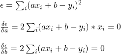
\\ \epsilon = \sum_i (a x_i + b - y_i)^2 \\ \\ \frac{\delta\epsilon}{\delta a} = 2 \sum_i (a x_i + b - y_i) * x_i = 0  \\ \\ \frac{\delta\epsilon}{\delta b} = 2 \sum_i (a x_i + b - y_i)  = 0

The above equations lead to two sets of linear equations that need to be solved.

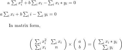
\\  a \sum_i  x_i^2 + b \sum_i  x_i  - \sum_i  x_i *y_i  = 0  \\ \\  a \sum_i  x_i + b \sum_i  i  - \sum_i y_i  = 0  \\  \text{ In matrix form, } \\  \[ \left( \begin{array}{cc} \sum_i  x_i^2 &  \sum_i  x_i \\ \sum_i  x_i &  n  \end{array} \right) \times  \[ \left( \begin{array}{c} a \\  b  \end{array} \right) = \[ \left( \begin{array}{cc} \sum_i  x_i*y_i \\ \sum_i  y_i  \end{array} \right)

We solve this equation for a and b using the following r code


Q1 <- data.frame("x" = c(10, 8, 13, 9.0, 11.0, 14.0, 6.0, 4.0, 12.0, 7.0, 5.0), "y" = c(8.04, 6.95, 7.58, 8.81, 8.33, 9.96, 7.24, 4.26, 10.84, 4.82, 5.68))

x_i_2  <-  sum(Q1$x*Q1$x)
x_i  <-  sum(Q1$x)
nn <- nrow(Q1)

x_i_y_i <- sum(Q1$x*Q1$y)
y_i <- sum(Q1$y)


X <- matrix(c(x_i_2, x_i, x_i, nn), 2, 2, byrow=TRUE)
y <- c(x_i_y_i,y_i)

solve(X, y)

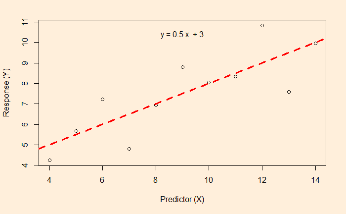
We get a = 0.5 (slope) and b = 3.0 (intercept). Now use the shortcut R code (“lm“) to verify

mm <- lm(Q1$y ~ Q1$x)

summary(mm)
Call:
lm(formula = Q1$y ~ Q1$x)

Residuals:
     Min       1Q   Median       3Q      Max 
-1.92127 -0.45577 -0.04136  0.70941  1.83882 

Coefficients:
            Estimate Std. Error t value Pr(>|t|)   
(Intercept)   3.0001     1.1247   2.667  0.02573 * 
Q1$x          0.5001     0.1179   4.241  0.00217 **
---
Signif. codes:  0 ‘***’ 0.001 ‘**’ 0.01 ‘*’ 0.05 ‘.’ 0.1 ‘ ’ 1

Residual standard error: 1.237 on 9 degrees of freedom
Multiple R-squared:  0.6665,	Adjusted R-squared:  0.6295 
F-statistic: 17.99 on 1 and 9 DF,  p-value: 0.00217

The original scatter plot with the model line included

Regression: The OLS Way Read More »

Outliers

Outliers are data points that don’t fit the model well. Outliers are data points that don’t fit the model well. Let’s take the previous example we did earlier.

Here is an updated dataset with the addition of a new point corresponding to x = 13 but doesn’t make sense to the otherwise overall behaviour.

You can see that the outlying data has pulled the right side of the regression line up.

Outliers Read More »