It would be interesting to see how the probability matrix is transformed as the number of stages progresses. Here is the original matrix (P), followed by (P10).
0.8  0.2  0.1
0.1  0.7  0.3
0.1  0.1  0.6
0.45 0.45 0.45
0.35 0.35 0.35
0.20 0.20 0.20
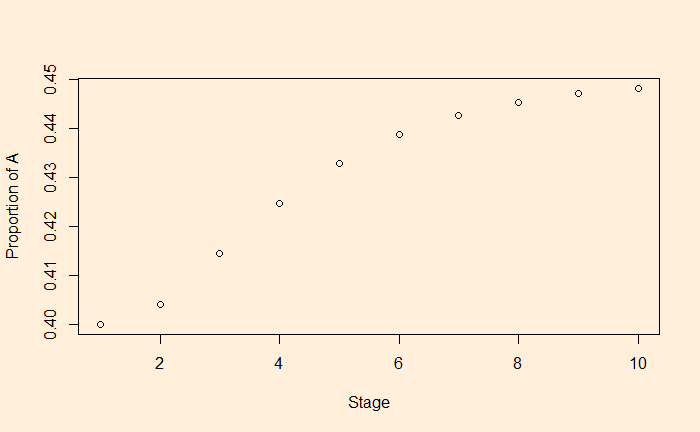
Elements in each raw are similar in magnitude, which suggests why the end result after multiplying it with the original proportion is the same after each stage.
Another interesting fact is how Xn changes with the initial proportion, X0. We use the following X0 values. Note that the sum of the proportions must add to 1.
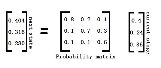
Last time, we saw how the next stage is developed from the current stage using the probability matrix.
X1 = P X0
There is a reason why it is called the Markov chain. The system we have developed can now predict the stage after the next stage, i.e., X2. Multiply the probability matrix with X1.
X2 = P X1
Substituting for X1, X2 = P P X0 X2 = P2 X0 or in general Xn = Pn X0
Let’s work out the stage after 10 moves and plot and see where A ends up.
In the last post, we started an example to demonstrate the objective of Markov processes.
The question is, what is the expected number of customers in shops A, B, and C in the following week?
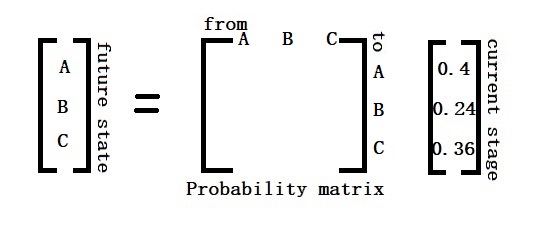
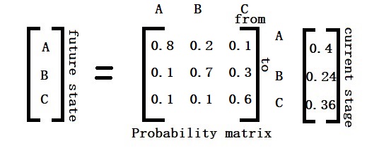
The whole formulation is nothing but future state = present state x a probability matrix. The probability matrix, fundamental to making this translation, is developed from the diagram we created earlier.
The first row of the matrix are the probabilities: A to A, B to A and C to A The second row: A to B, B to B and C to B The third row: A to C, B to C and C to C
Perform the matrix multiplication between the two. Here are the R codes.
The Markov approach is a concept for predicting stochastic processes. It models a sequence in which the probability of the following (n+1) event depends only on the state of the previous (n) event. Therefore, it is also called a ‘memoryless’ process.
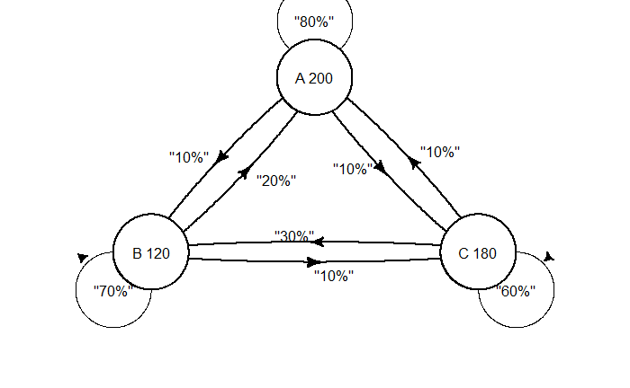
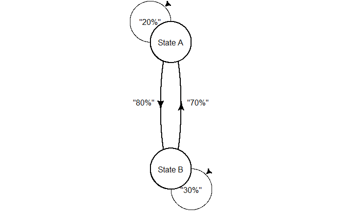
Before performing calculations, let’s familiarise ourselves with the concept and notations. Suppose there are two states: state A and state B. The process is expected to stay in the same stage for 20% of the time and can move to stage B in the remaining 80%. On the other hand, stage B has a 30% chance of staying and a 70% chance of moving to stage A. The following diagram depicts the process.
For example, imagine three shops in town—A, B, and C—that attract 200, 120, and 180 customers, respectively, this week. The following possibilities are expected for next week.
Shop A: 80% of the customers stay loyal 10% can move shop B 10% can move shop C
Shop B: 70% of the customers stay loyal 20% can move shop A 10% can move shop C
Shop C: 60% of the customers stay loyal 10% can move shop A 30% can move shop B
The question is, what is the expected number of customers in shops A, B, and C in the following week?
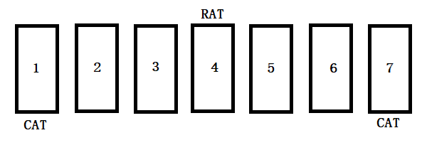
There are seven doors, and a mouse is at door 4. Two cats are waiting at door 1 and door 7. The rat moves one door in a day—either to the left or to the right. When it reaches the cat door, it gets eaten by the cat. What is the average number of days before the rat gets caught?
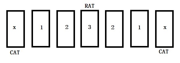
We can rename the arrangement since the mouse sits in the middle of the door sequence.
In the beginning, the mouse is at door 3, and let e3 be the expected time until the mouse gets caught by the cat. After one day, the mouse has a 50% chance of reaching the left or a 50% chance of reaching the right door. Either way, it reaches door 2 and lets e2 be the expected time until caught. Therefore,
e3 = 1 + e2
When the rat is one 2, after one day, the mouse has a 50% chance of reaching door 3 (waiting time e3) or a 50% chance of reaching door 1 (waiting time e1).
e2 = 1 + 0.5 e3 + 0.5 e1
From there, it either reaches door 2 or gets caught in a day.
e1 = 1 + 0.5 e2
Now, we have three linear equations to solve. e3 = 1 + e2 e2 = 1 + 0.5 e3 + 0.5 e1 e1 = 1 + 0.5 e2
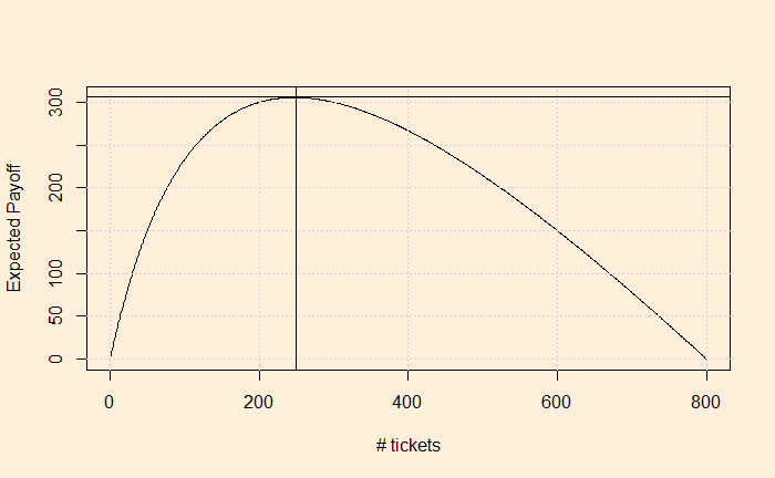
Amy walks into a raffle house and finds it about to close. They are raffling off an object with a value of $1000. She finds that only 200 tickets have been sold. Knowing they will draw the winner at any time, how many tickets should Amy purchase to maximise the expected value? The cost is $1 per ticket.
The expected payoff = expected value of the lottery – the price you paid. = value of the object x the probability of winning – the price you paid. the probability of winning = # ticket you bought / total # tickets sold.
If x is the number of tickets Amy purchased, The expected payoff = [1000 * x /(200 + x)] – x
So, we need to find the x that maximises the payoff. One way to determine is to plot the expected payoff ([1000 * x /(200 + x)] – x) as a function of the # tickets (x) you purchased and see where it maximises.
The number of tickets that maximises the expected payoff is somewhere close to 250.
It is a binary game similar to a coin toss. Player 1 selects a sequence (of length 3 or larger) first, followed by Player 2. The player whose sequence comes up first wins. The question is, can player 2 maximise her chance?
Apparently, Player 2 can always select a sequence based on what Player 1 has already picked that can maximise her winning odds. It is based on a simple strategy. The second player looks at Player 1’s sequence and picks the opposite of the middle one to start with, followed by the first player’s first two choices.
In the last post, we saw how CVD incident rates have increased since the start of the pandemic and the possible reasons for this. Today, we examine why the vaccine—and not COVID itself—has become the principal offender in the common belief.
Chemophobia
Blame it on the ‘silent spring’, the Bhopal tragedy, or Chornobyl; chemophobia, or the fear of chemicals, is real. We have seen how heuristics or mental shortcuts play a role in decision-making. Studies found that most of us, the non-experts of toxicology, tend to rely on heuristics when judging chemical safety. The public leans on three ‘rules of thumb’ when evaluating chemicals. Natural-is-better heuristics: People associate better confidence in dealing with natural substances than synthetic ones. It may sound incredible, but people find it more comfortable trusting a herb containing 10,000 unknown molecules than a well-researched single compound drug when dealing with a medical condition. The reason? – one is natural, and the other is made. It goes to such an extent that in one study, Siegrist and Bearth found that only 18% of the people surveyed thought the chemical structures of synthetically prepared and naturally occurring NaCl were identical. Contagion heuristics: These come from a lack of knowledge of the concept of dose. People view a chemical as either safe or toxic while missing out on the quantity. For the decision maker (the brain), this keeps the decisions simple. In the same survey, three-quarters of the people believed that a toxic substance is always dangerous irrespective of its dose. Trust heuristics: States that people rely on their trust (or lack thereof) in key stakeholders, such as chemical industries and governmental and non-governmental organisations, to evaluate the associated risk.
For ordinary people, the leading COVID-19 vaccines—Moderna, Pfizer, and Oxford—were all human-made. Therefore, they are dangerous. On top of this, thanks to the ever-vigilant regulators in the EU and the US, the side effects of vaccines—that they could cause severe blood clots or myocarditis in a few in a million people—were public within a few months of their introduction.
Affirming the consequent
Irwin, the hypochondriac: “I’m sure I have liver disease.” “That’s impossible”, replied the doctor. “If you have liver disease you’d never know it.” Irwin replies: “Those are my symptoms exactly.”
Rationality by Steven Pinker
Affirming the consequent is a formal logical fallacy of the following type. IF P, THEN Q. Q. Therefore, P.
In the case of the vaccine, the logical fallacy works this way: A. Vaccines cause myocarditis and pericarditis in some. B. The patient had a heart attack. C. It must be the vaccine.
Not familiar with the risk-benefit trade-off
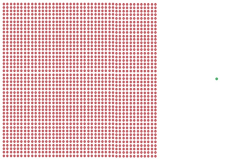
No decision is risk-free, and medication is no exception. The important thing is to evaluate the risk caused by an action compared to a situation without that action. That is the core of the risk-benefit trade-off in decision-making. And the risks due to vaccination must be viewed that way. I will end with the scheme we developed at the peak of the pandemic.
Death due to Infection (red) vs Death by Vaccine (green)
References
[1] Siegrist, M., Bearth, A. Chemophobia in Europe and reasons for biased risk perceptions. Nat. Chem. 11, 1071–1072 (2019). https://doi.org/10.1038/s41557-019-0377-8 [2] Steven Pinker, Rationality, Penguin Random House
The World’s leading cause of death is cardiovascular diseases (CVDs) – heart attacks and strokes. Globally, the estimated number of deaths due to CVDs increased from around 12.1 million in 1990 to 18.6 million in 2019. Note that the age-standardised death rate has declined from 354.5 deaths per 100,000 people in 1990 to 239.9 deaths per 100,000 people in 2019. While pollution, unhealthy diet, alcohol and tobacco are the leading root causes, the increase in the absolute number of CVD deaths is primarily due to growth in population and life expectancy.
Against this backdrop, we examine the anomalies in death rates in the last five years. According to CDC data, heart diseases accounted for 702,880 deaths in the US in 2022. Here is the figure representing the trend from 2018 to 2022.
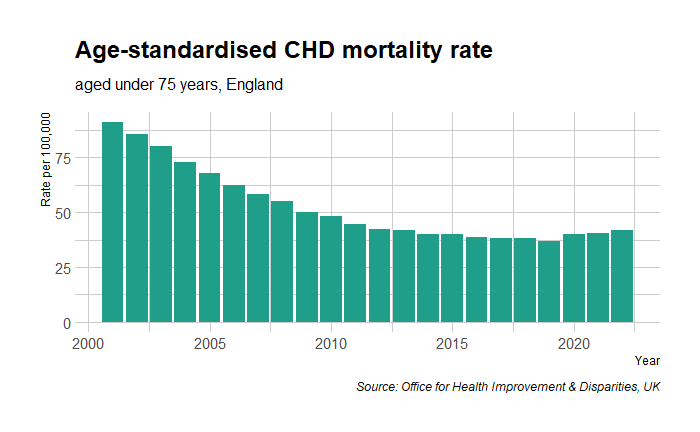
Contrary to trends in the last few decades, the death rates jumped from 200 to 211 from 2019 to 2020. Notably, 2020 also marked the start of the global pandemic, COVID-19. The story was no different for the rate of mortality from Coronary Heart Disease (CHD) in England.
Hypothesis on test
Let’s examine the two hypotheses to explain this rise in deaths due to the pandemic. 1) Covid-19 played a role, and 2) Covid vaccine played a role. We will start with the easier one – the vaccine.
The authorisation of leading vaccines – Moderna, Pfizer and AstraZeneca – for first use happened in December 2020, and the active vaccination program only started months later. Note that the ‘jump’ occurred from 2019 to 2020, a year earlier than the start of vaccination.
Now, the impact of COVID-19 on heart disease. Again, there are two possibilities: the virus directly causes heart disease, or the virus is part of the causal chain (VIRUS—MEDIATOR—CVD). Data suggest that there is evidence for the first possibility. While COVID-19 is a risk modifier—something that worsens pre-existing CVD risk factors such as hypertension—heart attacks are only the fourth or fifth cause of death in COVID-19 patients, respiratory failure being the leading cause.
The elephant in the room
The British Heart Foundation published a report in 2022 that summarises their investigation of the excess deaths due to CVD after the pandemic breakout. They found that COVID-19 infection alone was not sufficient to explain the 14% increase in ischaemic heart disease (IHD) compared to the pre-pandemic period. Instead, the breakdown of the healthcare system was the likely cause. The team surveyed and found
43% of patients who needed medical treatment for their heart condition have put off seeking NHS help due to ongoing fears of catching Covid or burdening NHS services.
20% of heart patients reported having had an appointment for their heart condition cancelled over the last year.
The proportion of patients with diagnosed hypertension who had their BP checked fell from 89% in March 2020 to 64% by March 2021.
Two million fewer people were recorded as having controlled hypertension in 2021 compared to the previous year.
Modelling from NHSE shows that this reduction in blood pressure control could lead to an estimated 11,190 additional heart attacks and 16,702 additional strokes over three years.
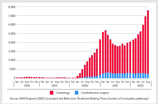
Here is a trend of the number of patients waiting for treatment (source: NHS England)
The picture is no different for heart procedures. (Source: NHS England (2022) Consultant-led Referral to Treatment Waiting Times (number of incomplete pathways)):
Another study published in Nature Medicine used monthly counts of prevalent and incident medications dispensed and found a systematic trend of decline, especially during the lockdown periods.
In summary
Managing cardiovascular diseases requires constant action via public health agencies. These include detection, consultations, medications, and procedures. The COVID pandemic has temporarily affected the flow of this machinery, and the result was an increase in CVD mortality. Yet, the public perception focused on vaccines. Why did that happen? We’ll see that next.
[3] Elezkurtaj, S., Greuel, S., Ihlow, J.hospitalisedes of death and comorbidities in hospitalised patients with COVID-19. Sci Rep11, 4263 (2021). https://doihospitalised/s41598-021-82862-5
[4]Dale, C.E., Takhar, R., Carragher, R. et al. The impact of the COVID-19 pandemic on cardiovascular disease prevention and management. Nat Med29, 219–225 (2023). https://doi.org/10.1038/s41591-022-02158-7
[5] Vosko, I., Zirlik, A., Bugger, H., Impact of COVID-19 on Cardiovascular Disease, Viruses, 15(2), 508 (2023).