Data & Statistics

Confusion Matrix

Machine learning is a technique to train a model (algorithm) using a dataset for which we know the outcome and then use the algorithm, making predictions where we don’t have the outcome. The confusion matrix is the summary in a tabular form, highlighting the model performance.
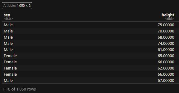
Height data

We develop a simple machine learning algorithm predicting the sex of a person from the height data. The R package to help here is ‘caret’. Here are the first ten entries of the dataset that contains 1050 members.

The first thing is to check whether we can distinguish between the heights of males and females. The following command summarises the mean and standard deviation of heights.

heights %>% group_by(sex) %>% summarize(Mean = mean(height), SD = sd(height))

Yes, the males are a little taller than the females, and we use this property to make decisions. I.e., assign the output as male if the height is greater than 64 inches and female otherwise. But before getting into the calculations, we divide the dataset randomly into two halves – training set and test set – using the ‘createDataPartition’ in the ‘caret’ package.

test_index <- createDataPartition(heights$height, times = 1, p = 0.5, list = FALSE)
train_set <- heights[-test_index,]
test_set <- heights[test_index,]

Now, we have two sets with 526 members each. We apply the algorithm to the training set and see the results.

y_hat <- ifelse(train_set$height > 64, "Male", "Female") %>%  factor(levels = levels(train_set$sex))
mean(y_hat == train_set$sex)

We apply the formulation to the test set and get the confusion matrix.

y_hat <- ifelse(test_set$height > 64, "Male", "Female") %>% 
  factor(levels = levels(test_set$sex))

confusionMatrix(data = y_hat, reference = test_set$sex)
Confusion Matrix and Statistics

          Reference
Prediction Female Male
    Female     55   24
    Male       64  383
                                         
               Accuracy : 0.8327         
                 95% CI : (0.798, 0.8636)
    No Information Rate : 0.7738         
    P-Value [Acc > NIR] : 0.0005217      
                                         
                  Kappa : 0.4576         
                                         
 Mcnemar's Test P-Value : 3.219e-05      
                                         
            Sensitivity : 0.4622         
            Specificity : 0.9410         
         Pos Pred Value : 0.6962         
         Neg Pred Value : 0.8568         
             Prevalence : 0.2262         
         Detection Rate : 0.1046         
   Detection Prevalence : 0.1502         
      Balanced Accuracy : 0.7016         
                                         
       'Positive' Class : Female         
                                    

In the tabular form,

Actual
FemaleMale
PredictedFemale5524
Male64383

The rows on the confusion matrix present what the algorithm predicted, and the columns correspond to the known truth. The output provides a bunch of other metrics. That is next.

Confusion Matrix Read More »

BreakUp Drinking

Here is the data on alcohol consumption before and after the breakup. There is an assumption that the drinking habit increases post-breakup. Is that true?

BeforeAfter
470408
354439
496321
351437
349335
449344
378318
359492
469531
329417
389358
497391
493398
268394
445508
287399
338345
271341
412326
335467

The null hypothesis, H0: (consumption after – before) = 0.
The alternative hypothesis, HA: (consumption after – before) > 0.

T-Test

\textrm{T-Statistic } = \frac{D - \mu_d}{S_d/\sqrt{n}}

D = Mean difference of the parameter after and before
mud = hypothesised mean difference
Sd = Standard deviation of the difference
n = number of samples

We insert the data in the following command and run the function, t.test.

Before <- c(470, 354, 496, 351, 349, 449, 378, 359, 469, 329, 389, 497, 493, 268, 445, 287, 338, 271, 412, 335)

After  <- c(408, 439, 321, 437, 335, 344, 318, 492, 531, 417, 358, 391, 398, 394, 508, 399, 345, 341, 326, 467)

t.test(Before, After, paired = TRUE, alternative = "greater")
	Paired t-test

data:  Before and After
t = -0.53754, df = 19, p-value = 0.7014
alternative hypothesis: true mean difference is greater than 0
95 percent confidence interval:
 -48.49262       Inf
sample estimates:
mean difference 
          -11.5 

There was a difference of -11.5, yet the p-value (0.7014) is higher than the critical value we chose (0.05). The test shows no evidence supporting the hypothesis.

BreakUp Drinking Read More »

The Nocebo Effect

A placebo is used in clinical trials as a control in drug studies to test the effectiveness of treatments. In drug trials, one group of participants receives the medicines (to be tested), and the other gets the placebo (say, sugar pills).

The concept of placebo stems from the assumption that a treatment has two components, one related to the specific effects of the treatment and the other, nonspecific, related to its perception. When the nonspecific effects are beneficial to the participant, it is called a placebo, and when they are harmful, it is a nocebo.

Hypothesis Testing

The null hypothesis (H0) typically represents the default state or the state of “no effect“. For example, you compare the means of two groups, such as people who took a particular drug and people who received the placebo. As a drug researcher, your objective is to find the effectiveness of the medicine. And that lays the foundation for your alternative hypothesis (HA or H1) – that the drug has a non-zero effect. The default state (H0) assumes the drug has no impact. To be specific, H0 assumes the difference between two means equals zero.

The Nocebo Effect Read More »

Decision Trees

Decision trees are logical pathways created by tracing answers to multiple stages of true/false, no-go/no-go questions. Here is a representation of a simple tree based on a person liking something given their age.

Another to represent the same info is:

A regression tree is a type of decision tree. In the regression tree, each leaf represents a numeric value. The other type is a classification tree with true/false or another category in its leaves.

Decision Trees Read More »

Power of a Statistical Test

The power of a statistical test is the probability of rejecting the null hypothesis when the null hypothesis is false (or the effect is present). It is the right decision, and before we go deeper into it, let’s recap the two types of errors in hypothesis testing.

  1. A type I error is when the Null hypothesis is true, but you rejected it.
  2. A type II error is when you fail to reject a false Null hypothesis; in other words, the effect is present.

In a tabular format,

Null hypothesis (H0)
is TRUE
Null hypothesis (H0)
is FALSE
FAIL to RejectCorrect Decision
(probability = 1 – α)
Type II Error
(probability = β)
Reject Type I Error
(probability = α)
Correct Decision
(probability = 1 – β)

Your guess is right, Power equals 1 – β.

Power of a Statistical Test Read More »

Two Sample Proportions Test – Effect of Sample Size

Amelie has developed a new drug against the flu and wanted to test its effectiveness. She recruited 50 people and divided them into two groups. She gave the medicine to the first group (34 people) and provided a placebo to the second (16). Here are the results.

In the treatment group, 15 out of 34 (44%) recovered in 1 day.
In the control group, 4 out of 16 (25%) recovered in 1 day.

Amelie thinks her medicine is effective because of the big defence (44 – 25 = 19%) in performance and the larger sample size for the treatment group. Do you agree?

We must do a statistical test to conclude. The data is:

SampleEventsTrials
Treatment1534
Control416

The Null Hypothesis, H0: No impact of medicine; recovery proportion on drug equals that of placebo.
The Alternative Hypothesis, H1: Medicine improves the condition; recovery proportion on drug greater than placebo.

We use the ‘prop.test()’ function in R.

prop.test(x = c(15, 4), n = c(34, 16), alternative = "greater")

We used the one-tailed test to determine whether the treatment has improved the condition compared to the control.


	2-sample test for equality of proportions with continuity correction

data:  c(15, 4) out of c(34, 16)
X-squared = 0.97389, df = 1, p-value = 0.1619
alternative hypothesis: greater
95 percent confidence interval:
 -0.0813273  1.0000000
sample estimates:
   prop 1    prop 2 
0.4411765 0.2500000 

The p-value of 0.1619 (more than the significance value of 0.05) is not enough to reject the null hypothesis.

What would have happened if she had recruited more people in the placebo group and found results at the same proportions?

SampleEventsTrials
Treatment1534
Control1664
prop.test(x = c(15, 16), n = c(34, 64), alternative = "greater")
	2-sample test for equality of proportions with continuity correction

data:  c(15, 16) out of c(34, 64)
X-squared = 2.9205, df = 1, p-value = 0.04373
alternative hypothesis: greater
95 percent confidence interval:
 0.002691967 1.000000000
sample estimates:
   prop 1    prop 2 
0.4411765 0.2500000 

Here, the results are significant (p-value = 0.04373 < 0.05) to reject the null hypothesis in favour of the alternate (that the drug works).

What about recruiting more to the treatment group?

SampleEventsTrials
Treatment150340
Control416
prop.test(x = c(150, 4), n = c(340, 16), alternative = "greater")
	2-sample test for equality of proportions with continuity correction

data:  c(150, 4) out of c(340, 16)
X-squared = 1.5631, df = 1, p-value = 0.1056
alternative hypothesis: greater
95 percent confidence interval:
 -0.02503096  1.00000000
sample estimates:
   prop 1    prop 2 
0.4411765 0.2500000 

p-value = 0.1056; the null hypothesis stays!

Or, had many individuals in both groups?

SampleEventsTrials
Treatment150340
Control40160
prop.test(x = c(150, 40), n = c(340, 160), alternative = "greater")
	2-sample test for equality of proportions with continuity correction

data:  c(150, 40) out of c(340, 160)
X-squared = 16.076, df = 1, p-value = 3.042e-05
alternative hypothesis: greater
95 percent confidence interval:
 0.1149402 1.0000000
sample estimates:
   prop 1    prop 2 
0.4411765 0.2500000 

Both the groups have plenty of samples, and now the difference (44 – 25 = 22%) overwhelmingly supports the impact of the medicine.

Two Sample Proportions Test – Effect of Sample Size Read More »

Margin of Error – Continued

In the previous post, we saw how the margin of error at a specified confidence interval is estimated. The margin of error, and thereby the confidence in the data, varies with the number of samples and the confidence interval.

Here are five calculations with varying numbers of samples (500, 1041 and 2000) for three confidence intervals (90%, 95%, 99%).

As the sample size increases, the margin of error decreases, i.e., the more people you survey, the more confident you can be that your results are closer to the “true” population value (provided the sample is representative). However, the reduction diminishes as the sample size goes beyond 1000.

Margin of Error – Continued Read More »

Margin of Error

A recent study suggests that 63% of the people in a city believe in parapsychological phenomena. The study surveyed 1041 residents. What is the margin of error of the results at a 95% confidence interval?

This is the problem of estimating the margin of error on point estimates from a sample. You may know by now that the ultimate goal is to calculate the population proportion, for which sampling (and thus obtaining the sample proportion) is the only practical path. The point estimate of proportion, p, is evaluated from x, the number of successes (people who said “YES” to parapsychology here), and the sample size (n):
p = x/n

The remaining, 1 – p, is the proportion of failures (n – x out of n).

In the given sample, 0.63 is the p or the proportion of people who believed in parapsychology. Can you conclude that 0.63 remains the fraction of similar believers in the city? The answer is No; therefore, we estimate the margin of error by applying the formula. The margin of error gives the expected range of values to capture the population at some confidence level.

margin of error = z-critical value x square root (p x (1-p) / n)

MoE = z_{\alpha/2} \sqrt{\frac{p (1-p)}{n}}

z-critical value for a 95% confidence interval is 1.96, for 99% is 2.576, etc.

The whole process can be done in one step using R.

prop.test(proportion*n_sample, n_sample, p = NULL, alternative = "two.sided",
          correct = TRUE, conf.level = 0.95)
	1-sample proportions test with continuity correction

data:  proportion * n_sample out of n_sample, null probability 0.5
X-squared = 69.853, df = 1, p-value < 2.2e-16
alternative hypothesis: true p is not equal to 0.5
95 percent confidence interval:
 0.5997570 0.6592715
sample estimates:
   p 
0.63 

Or by applying the formula directly.

n_sample <- 1041
proportion <- 0.63

std_error <- sqrt(proportion*(1-proportion)/n_sample)
margin <- std_error*qnorm(0.975)
proportion + margin
proportion - margin

The margin of error is 0.029, and the confidence interval is found by adding and subtracting it from the sample proportion (0.63).

[ 0.600, 0.659]

So, we are 95% confident that the true proportion of the population lies between 0.600 and 0.659, right? Not really; it only means that if you perform several random samples from this population, we expect about 95% of those intervals to contain the true proportion.

Margin of Error Read More »

Anthropic Principle

The anthropic principle says that in the universe, our presence as observers compels conditions for our presence. While the idea was not entirely new, the phrase came up in 1973 by Brandon Carter, who proposed the weak and strong forms of anthropic principle.

The weak anthropic principle (WAP) merely says that you need to take into account those things in the environment that you can see vs those things you are unable to see. Or it simply says that the life-free universes cannot be observed it’s just a selection bias.

An example is the cosmological constant (lambda). The number must be within certain limits. If the constant were large-negative, the universe would have collapsed long ago; if it were large-positive, it would have expanded too fast for the stars to form. Either way, we wouldn’t be here to talk about it.

Anthropic Principle Read More »