Data & Statistics

Drunken Man and the Room Key – Simulations

Here is the simulation of the problem of the drunken man and keys. Let me repeat the problem statement: A drunk man reaches his home and tries the door key from a bunch of 10 keys. If the first key doesn’t work, he returns the key to the bunch and randomly selects another key repeatedly until he opens the door. The question is: which precise trial has the highest probability of opening the door?

library(reshape)
library(ggplot2)

key <- 3
itr <- 100000

drunk <- replicate(itr, {
index <- 1
    for(i in 1:100) {
    sel <- sample(seq(1:10), 1, replace = TRUE, prob = rep(1/10,10))  
if(sel == key){
 index 
 break 
}else{
  index = index + 1
}
    }
index
    })

temp.melt <- melt(table(drunk))

ggplot(temp.melt, aes(x = drunk, y = value/itr)) +
  theme_bw() +
  geom_bar(stat = "identity", fill = "brown") +
  xlim(0,20) +
 
labs(x= "Attempt #",
       y= "Probability") +
  theme(legend.position="none") +

theme(text = element_text(color = "black"), 
        panel.background = element_rect(fill = "antiquewhite1"), 
        plot.background = element_rect(fill = "antiquewhite1"),
        panel.grid = element_blank())

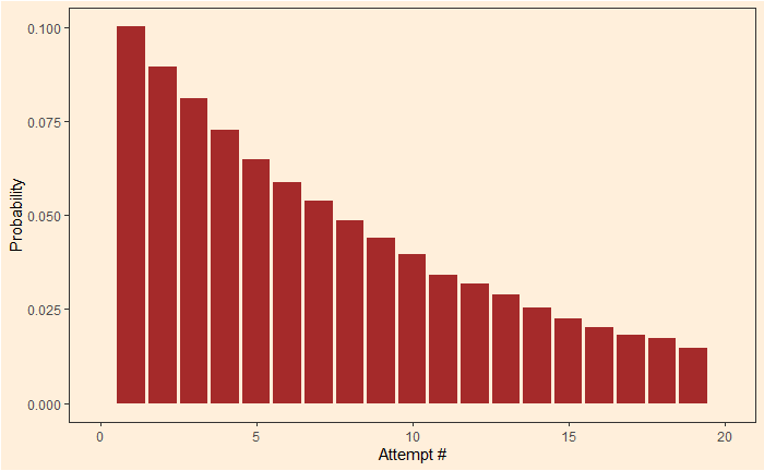
Drunken Man and the Room Key – Simulations Read More »

Drunken Man and the Room Key

Here is an interesting but misleading probability question: A drunk man reaches his home and tries the door key from a bunch of 10 keys. If the first key doesn’t work, he returns the key to the bunch and randomly selects another key repeatedly until he opens the door. The question is: which precise trial has the highest probability of opening the door?

The question is misleading because it does not ask you to guess by which try the person will find the right key and open the door. We’ll come to that topic a little later. The task is to find the probability of finding the right key at each try and show which one is the highest.

The probability of finding the right key in his first attempt = 1/10; ten keys and finding one at random is one out of 10 possible options.
The probability of finding the right key in his second attempt = (9/10)x(1/10); it is the joint probability of not getting the right key in the first attempt (9/10) AND the chance of hitting the right on the second try.
The probability of finding the right key in his third attempt = (9/10)x(9/10)x(1/10). Here is the summary:

AttemptProbability
10.1
20.09
30.081
40.0729
50.06561

It doesn’t mean that person will open the door in the first attempt or never. We need to estimate something different to find how the probability of opening the door changes with attempts. The chance he opened the door in his second attempt is:
Probability he opened in the first OR probability he opened in the second = 1/10 + (9/10)*(1/10). Here is how that develops.

AttemptProbabilityProbability of
Right key by
Attempt
10.10.1
20.090.19
30.0810.27
40.07290.34
50.065610.41
60.0590.47

There is about a 50% chance he will open the door by his sixth attempt.

Drunken Man and the Room Key Read More »

Monthly Miracle

During the time that we are awake and actively engaged in living our lives, roughly for eight hour each day, we see and hear things happening at a rate of about one per second. So the total number of events that happen to us is about thirty thousand per day, or about a million per month. With few exceptions, these events are not miracles because they are insignificant. The chance of a miracle is about one per million events. Therefore we should expect about one miracle to happen, on the average, every month

Freeman Dyson

Morgan Housel’s latest book, Same as Ever’, continues from where he left off in his earlier very popular, “The Psychology of Money”. It’s about human psychology and its inability to comprehend probability.

The brain always craves certainty or a black-or-white world. And even trained people find it challenging to reconcile with the math behind chances. The lottery winning odds, as perceived by journalists in the last post, is just one example of that. The result is that newspapers continue to display shocking headlines, reinforcing people’s trust in magic and divine interventions.

Here is an example: in a world with 8 billion humans, how many rarest of rare events, i.e., something with a probability of occurrence of once in a billion in a year, happens in a year? It seems difficult to imagine 8 billion people interacting with their surroundings is analogous to 8 billion independent binomial trials:

P(s; p, n) = nCs x ps (1-p)n-s

The formula represents the probability of s number of ‘success’ if n number of independent trials happen, each with a chance of p. In our problem, substitute n with 8 billion and p with 1/1,000,000,000.

The probability of no ‘miracle’ happening in a year, i.e., s = 0.

P(0; 1×10⁻⁹, 8×10⁹) = 1 x 1 x (1-1×10⁻⁹)8e9

The answer is almost ZERO; subtracting 10-9 from 1 gives a fraction just short of 1, which multiplies by itself a few billion times, and the answer leads to nearly nothing.

You can evaluate the formula for s = 1, 2, etc. We will use the R function for that and plot.

s <- seq(0,15)
plot(s, dbinom(s, 8e9, 1e-9))

There is more than a 10% chance to see 5, 6, 7, 8, 9 or 10 miracles in a given year. The only thing is: it can’t say where it will happen; it will happen somewhere, and the journalist will dig it up to her headlines.

Monthly Miracle Read More »

Coincidences and A Double Lottery Winner

In 1985, Evelyn Marie Adams won $3.9 million in the New Jersey lottery. Four months later, in 1986, she won again; it was $1.4 million this time! The New York Times ran an article claiming that the probability of such an event was one in 17 trillion. Their argument must have been:

The probability of winning the first lottery – 6 numbers out of 39:
1/39C6 = 1/3262623
The probability of winning the first lottery – 6 numbers out of 42:
1/42C6 = 1/5245786
The chance of her winning both = (1/3262623)x(1/5245786) = 1/17 x 1012

This was actually the correct answer to a wrong question. The question should have been:
What is the probability that both tickets will be winners if you buy precisely two tickets for the New Jersey state lottery?”

Instead, the probability here was:
What is the chance that someone, out of millions of people buying lottery tickets each week in the United States, hits the lottery twice in four months?

Stephen Samuels and George McCabe of the Department of Statistics at Purdue University, who wrote in the newspaper’s opinion column, estimated that to be 1 in 30.

Reference

More Lottery Repeaters Are on the Way: NYT

Coincidences and A Double Lottery Winner Read More »

Weibull and Rayleigh Distributions

We have seen Weibull before. It is a continuous probability distribution that finds applications in various fields, such as engineering and reliability analysis. It is because of the flexibility to adapt to different shapes: uniform, left, or right-skew.

The shape and scale are the names of two typical parameters in a Weibull distribution. Depending on their values, one can get shapes such as:

Shape between 1 and 2.6: Right-skewed

xx <- seq(0,20, 0.1)
plot(xx, dweibull(xx, shape = 2, scale = 4))

Shape ~ 3 Uniform

Shape > 3.7 Left-Skewed

The Rayleigh distribution is a special case of the Weibull distribution. Rayleigh has one parameter, namely the scale. If The Rayleigh scale parameter is A, the corresponding Weibull has a scale = sqrt(2)xA and shape = 2. Here is a comparison between Rayleigh and Weibull for a Rayleigh scale= 3.

xx <- seq(0,20, 0.1)
plot(xx, drayleigh(xx, scale = 3), type = "l", ylim = c(0,0.25), lwd = 3, xlab = "X", ylab = "Density")
lines(xx, dweibull(xx, shape = 2, scale = sqrt(2)*3), type = "l", ylim = c(0,0.25), col = "red", lwd = 5, lty=3)

Here, Black represents the Rayleigh and red the Weibull.

Weibull and Rayleigh Distributions Read More »

Again Russian Roulette

Suppose a person is forced to play the Russian Roulette. Here is how it works: the person must try two, each time spinning a six-chambered revolver before pulling the trigger. He also gets two options to choose from: 

  1. A revolver with two bullets in it
  2. Randomly select one of the two revolvers – one carrying three bullets and the other with one bullet.
    Which is a better choice?

Let’s evaluate the survival chance of each:

1. Revolver with two bullets firing two times:
Probability survival after two rounds (randomised and made independent by spinning the barrel each time) = (4/6)x(4/6) = 0.44
2a. Revolver with three bullets:
(3/6)x(3/6) = 0.25
2b. Revolver with one bullet:
0.69

The chance of 2a or 2b to occur is 50:50. Therefore, the overall probability in the second case is (1/2) x (0.25 + 0.69) = 0.47

well, the second option gives a slightly better chance of survival!

Again Russian Roulette Read More »

Three Poisson Problems

The average number of bacteria per ml water is six. What is the probability of finding less than four bacteria in 1 ml of water?

This is an example of a problem that can be solved using the Poisson probability model. It involves a random variable, X, and it takes positive values. All we know is an expected value (average value), lambda. The probability is expressed as:

\\ P(X = s) = \frac{e^{-\lambda}\lambda^s}{s!}

In the bacteria problem, s is the total of all numbers less than four, i.e., 0+1+2+3 (P(X=0) + P(X=1) + P(X=2) + P(X=3). In R, it can be estimated as:

exp(-6)*6^0 / factorial(0) + exp(-6)*6^1 / factorial(1) + exp(-6)*6^2 / factorial(2) + exp(-6)*6^3 / factorial(3)
0.1512039

Even better: use the in-built function for the cumulative density function, ppois().

ppois(3,6, lower.tail = TRUE)

Recovery vehicle

There is a stretch of road in the city where, on average, five accidents happen during rush hour. The city council will purchase a recovery vehicle if the probability of having more than five accidents in the rush hour is more than 30%. Should the council go for a recovery vehicle?

Let’s use the R function:

ppois(5, 5, lower.tail = FALSE)

0.38

38% is above the cut-off value, so go for it!

Note that ppois(5, 5, lower.tail = FALSE) = 1 – ppois(5, 5, lower.tail = TRUE)

Birthday on Jan 1st

In a group of 30,000 married couples, what is the probability that at least one couple share their birthday on January 1?

Lambda, or the expected value, is the total number of couples x probability of a pair having the same given birthday. i.e., 30000 x (1/365) x (1/365) = 0.225.

At least 1 = 1 – P(X=0)

1 - dpois(0,0.225)
0.20

or

ppois(0, 0.225, lower.tail = FALSE)

Three Poisson Problems Read More »

Groomsmen and Bridesmaids

A couple wants to invite their friends to be at their wedding party. The party will consist of five groomsmen and five bridesmaids. The groom has eight possible groomsmen, and the bride has 11 bridesmaids.

1. How many groups are possible?

The order doesn’t matter, so it’s combinations.

_nC_r = \frac{n!}{(n-r)!r!}

For the groom, it becomes,

_8C_5 = \frac{8!}{(8-5)!5!} = \frac{8*7*6*5*4*3*2*1}{(3*2*1)*(5*4*3*2*1)} = 8*7 = 56

For the bride,

_{11}C_5 = \frac{11!}{(11-5)!5!} = \frac{11*10*9*8*7*6*5*4*3*2*1}{(6*5*4*3*2*1)*(5*4*3*2*1)} = 11*3*2*7 = 462

And the overall combinations are: 56 x 462 = 25872

choose(8,5)*choose(11,5)
25872

2. Suppose one possible groomsman and one possible bridesmaid refuse to be together; how many groups are possible?

First, we leave those and make groups:

choose(7,5)*choose(10,5) 
5292

Now, add the situation where that member from one side is present, and the one from the other is moving out (there are two instances).

choose(1,1)*choose(7,4)*choose(10,5) 
choose(1,1)*choose(7,5)*choose(10,4)  
8820
4410

Sum all up:

18522

Groomsmen and Bridesmaids Read More »

Standardised Data

The total annual deaths in Florida and Alaska are 131,902 and 2,116, respectively. The total population in Florida is 12,340,000, and Alaska’s is 530,000. How are death rates compared?

Crude mortality rate

The simplest thing to do here is to calculate the crude mortality rates by dividing the deaths by the population.

FloridaAlaska
Crude mortality rate
/100,000
131,902 x 100,000/12,340,000
= 1069
2,116 x 100,000/530,000
=399

The crude mortality ratio is 1069/399 = 2.68. Does that mean that the death rate is unusually high in Alaska?

Standardisation

The problem statement is: Do Alaskans (study population) have a higher mortality rate than the Floridians (standard population)?

Step 1: Mortality rate in the standard population – stratification by age group:

AgePopulationRate
/100,000
<5850,000284
5-192,280,00057
20-444,410,000198
45-642,600,000815
>652,200,0004425
Totals12,340,000
Data from Florida

Step 2: Use study population age distribution to find the expected rate

AgeRate in FloridaPopulation
Alaska
Expected
deaths
<528460,000284×60,000/100,000
= 170.4
5-1957130,00057×130,000/100,000
= 74.1
20-44198240,000198×240,000/100,000
= 475.2
45-6481580,000815×80,000/100,000
=65.2
>65442520,0004425×20,000/100,000
= 89
Total2256.7
Data from Florida

Step 3: Compare total expected deaths to actual deaths
Standardised Mortality Rate (SMR) = 2,256.7/2,116 = 1.07

SMR is close to 1; therefore, there is nothing unusual about the death rate in Alaska compared to Florida.

References

Confounding and Effect Measure Modification: BUMC

Standardised Data Read More »

Three Cards

A bag contains three cards – one is red on both sides, the second is white on both sides, and the third is red on one side and white on the other. Amy draws a card without looking and keeps it on the table. If the card is red face up, what is the probability that it’s also red on this hidden side?

Intuition tells the probability to be 1/2. The argument goes like this: if the side up is red, there are two equal possibilities for the hidden side – red or white. Therefore, it’s 1/2. A slightly different version of the same logic estimates that once the person sees it red, it shuts the options white-white card, leaving only two red-red and red-white. The card must be one out of two.

Conditional Probability

Let’s investigate the problem using conditional probability (the Bayes’ rule).

P(RR|Ru) represents the required probability, or the card is RR given R is up.

P(RR|R_u) = \frac{P(R_u|RR)P(RR)}{P(R_u|RR)P(RR) + P(R_u|RW)P(RW)}

P(Ru|RR) = probability of red up given RR is the selected card
P(RR) = Prior probability of choosing the RR card
P(Ru|RW) = probability of red up given RW is the picked card
P(RW) = Prior probability of selecting the RW card

P(Ru|RR) must be 1 as RR will always show red up
P(RR) = 1/3, as there are three cards to choose from
P(Ru|RW) = 1/2, there is a 50:50 chance for red to show up from an RW card
P(RW) = 1/3

P(RR|R_u)= \frac{1 * 1/3}{1 * 1/3 + 1/2 * 1/3} = \frac{2}{3}

Three Cards Read More »