The table shows that the sum 5 occurs 4 times, and 7 can occur 6 times (out of the 36 possibilities). So, the probability of getting a five before seven (as the sum) is 4/(4+6) = 40%.
A regular die has six sides, and the probability of getting a six is 1/6. If the die is modified so that the number 6 now appears to be half than usual (the frequency is halved), what is the probability of rolling a 6?
The question implies that the probability of getting 6 is half that of the other probabilities (1 to 5). Let p6 be the probability of rolling a six. Let p be the probability of rolling any other side.
For the die: 5 x p + p6 = 1 given p6 = p/2 5 x p + p/2 = 1 11p = 2 p = 2/11 p6 = p/2 = 1/11
The probability of rolling a six is not 1/12 but 1/11.
Amy and Becky are two friends invited to a 5-member committee meeting. What is the probability that they get seats next to each other if: 1. the member seats are arranged in a round table 2. the member seats are arranged in a row
Seated around a roundtable
Given that Amy is seated as denoted in the figure, Becky can sit next to her if she gets one of the two seats marked as Betty. In a random seating assignment case, the probability for that to happen is 2 out of 4 or the probability for the two seated side by side is 2/4 = 50%
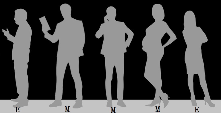
Seated in a row
As we did before, let’s place Amy first. In the end – two such places (E) In the middle – three such places (M)
Only one person can be next to the position E’s, but two positions are possible for M’s. A series of AND and OR rules estimate the overall possibility.
(Amy on E1 OR E2) AND (Becky on position 1) OR (Amy of M2 OR M3 OR M4) AND (Becky on position 1 OR Position 2). (1/5+1/5) x (1/4) + (1/5+1/5+1/5) x (1/4 + 1/4) 2/20 + 6/20 = 8/20 = 40%
Reference
How To Solve Bloomberg’s Random Seating Interview Question: MindYourDecisions
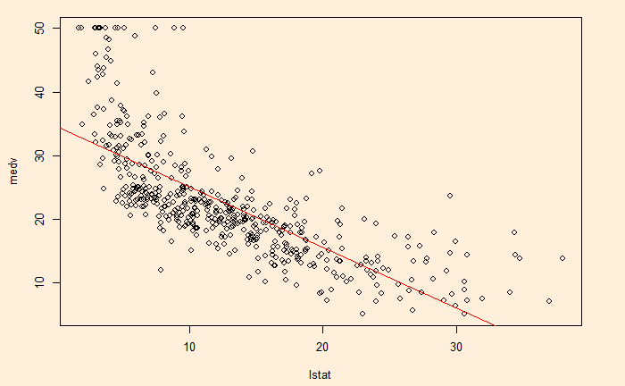
If you recall one of the previous posts relating ‘lstat’ with ‘medev’, we noticed the apparent curvature of the relationship. And how slightly awkward the fit-line on top of the scatter plot was.
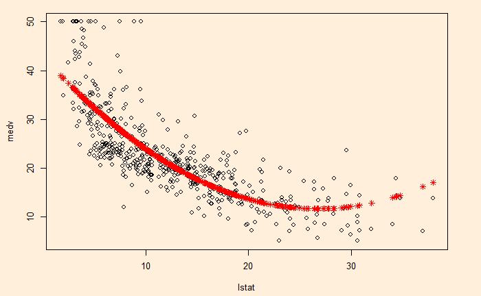
This seeming ‘non-linearity’ prompts us to extend the linear model to non-linear. We use a quadratic term by squaring the predictor (‘lstat’). We must use the identity function to do this.
fit5 <- lm(medv ~ lstat + I(lstat^2), Boston)
The results are presented below:
Call:
lm(formula = medv ~ lstat + I(lstat^2), data = Boston)

Residuals:
     Min       1Q   Median       3Q      Max
-15.2834  -3.8313  -0.5295   2.3095  25.4148

Coefficients:
             Estimate Std. Error t value Pr(>|t|)
(Intercept) 42.862007   0.872084   49.15   <2e-16 ***
lstat       -2.332821   0.123803  -18.84   <2e-16 ***
I(lstat^2)   0.043547   0.003745   11.63   <2e-16 ***
---
Signif. codes:  0 ‘***’ 0.001 ‘**’ 0.01 ‘*’ 0.05 ‘.’ 0.1 ‘ ’ 1

Residual standard error: 5.524 on 503 degrees of freedom
Multiple R-squared:  0.6407,	Adjusted R-squared:  0.6393
F-statistic: 448.5 on 2 and 503 DF,  p-value: < 2.2e-16
Now, let’s compare the fit results.
plot(medv~lstat, Boston)
points(Boston$lstat, fitted(fit5), col = "red", pch = 8)
Continuing from the previous post, we will add all the predictors in the regression this time. The notation is response variable ~ followed by ‘.’ [dot].
Which variables are better at predicting the response?
To answer the first question, we look at the results from two parameters, the R2 and F values. They both signify how the variance around the model is away from that around the mean. R-squared of 0.7343 and F-statistic = 113.5 are good enough to justify this activity.
The clues to the second question are also in the results (the stars at the end of the coefficients). The results show that two variables, ‘Indus’ and ‘age’, have very low significance (high p-values). So, we remove the least damaging predictors to the model and reevaluate using the ‘update’ command.
We have seen linear regression before as a simple method in supervised learning. It is of two types – simple and multiple linear regressions. In simple, we write the dependent variable (also known as the quantitative response) Y as a function of the independent variable (predictor) X.
Beta0 and beta1 are the model coefficients or parameters. You may realise they are the intercept and slope of a line, respectively. An example of a simple linear regression is a function predicting a person’s weight (response) from her height (single predictor).
Multiple linear regression
Here, we have more than one predictor. The general form for p predictors is:
We use the Boston data set from the library ISLR2 for the R exercise. The library contains ‘medv’ (median house value) for 506 census tracts in Boston. We will predict ‘medv’ using 12 predictors such as ‘rm’ (average number of rooms per house), ‘age’ (proportion of owner-occupied units built before 1940), and ‘lstat’ (per cent of households with low socioeconomic status).
First, we do the simple linear regression with one predictor, ‘lstat’.
fit1 <- lm(medv~lstat, Boston)
summary(fit1)
Call:
lm(formula = medv ~ lstat, data = Boston)

Residuals:
    Min      1Q  Median      3Q     Max
-15.168  -3.990  -1.318   2.034  24.500

Coefficients:
            Estimate Std. Error t value Pr(>|t|)
(Intercept) 34.55384    0.56263   61.41   <2e-16 ***
lstat       -0.95005    0.03873  -24.53   <2e-16 ***
---
Signif. codes:  0 ‘***’ 0.001 ‘**’ 0.01 ‘*’ 0.05 ‘.’ 0.1 ‘ ’ 1

Residual standard error: 6.216 on 504 degrees of freedom
Multiple R-squared:  0.5441,	Adjusted R-squared:  0.5432
F-statistic: 601.6 on 1 and 504 DF,  p-value: < 2.2e-16
Here is the plot with points representing the data and the line representing the model fit.
We will add another predictor, age, to the regression table.
fit2 <- lm(medv~lstat+age, Boston)
summary(fit2)
Call:
lm(formula = medv ~ lstat + age, data = Boston)

Residuals:
    Min      1Q  Median      3Q     Max
-15.981  -3.978  -1.283   1.968  23.158

Coefficients:
            Estimate Std. Error t value Pr(>|t|)
(Intercept) 33.22276    0.73085  45.458  < 2e-16 ***
lstat       -1.03207    0.04819 -21.416  < 2e-16 ***
age          0.03454    0.01223   2.826  0.00491 **
---
Signif. codes:  0 ‘***’ 0.001 ‘**’ 0.01 ‘*’ 0.05 ‘.’ 0.1 ‘ ’ 1

Residual standard error: 6.173 on 503 degrees of freedom
Multiple R-squared:  0.5513,	Adjusted R-squared:  0.5495
F-statistic:   309 on 2 and 503 DF,  p-value: < 2.2e-16
beta_0 is 33.22, beta_1 is -1.03 and beta_2 is 0.034. All three are significant, as evidenced by their low p-values (Pr(>|t|)). We will add more variables next.
An introduction to Statistical Learning: James, Witten, Hastie, Tibshirani, Taylor
Another counterintuitive experience similar to Downs–Thomson’s is Braess’s Paradox. As per this phenomenon, adding more roads to an existing network can slow down the overall traffic. Similar to the previous, we will see the mathematical explanation first.
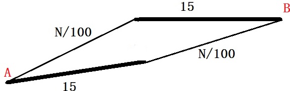
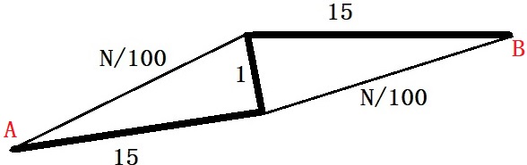
Suppose there are two routes to city B from city A, as shown in the picture – the top and bottom roads. The first part is narrow on the top road, followed by a broad highway. The situation is the opposite for the bottom road.
The highways are not impacted by the number of cars, whereas, for the narrower roads, the traffic time is related to the number of vehicles on the road – N/100, where N is the number of cars.
If there are 1000 cars in the city, the system will reach the Nash equilibrium by cars getting equally divided (in the longer term), i.e., 500 on each road. Therefore, each car to take 500/100 + 15 = 20 mins
Imagine a new interconnection built by the city to reduce traffic congestion. The travel time on the connection section is 1 minute. Let’s look at all scenarios.
Scenario 1: A car starts from the bottom highway, takes the connection, and moves to the top highway. Total time = 15 + 1 + 15 = 31 mins. Scenario 2: One car starts from the top road, takes the connection, and moves to the bottom road, while the others follow the old path (not using the connection). Total time = 50/100 + 1 + 51/100 ~ 11 mins.
Scenario 2 seems a no-brainer to the car driver. But this news invariably reaches everyone, and soon, everyone starts taking the narrow paths! In other words, the narrow route is the dominant strategy. The total travel time now becomes: 1000/100 + 1 + 1000/100 = 21 min. This is more than the old state, a situation with no connection possible.
So, the condition without the connection road (or closing down the connection road) seems a better choice. And this is Braess’s paradox suggesting that a more complex system may not necessarily be a better choice.
Here is a game theory puzzle for you. The government proposes to build a highway between the two cities, A and B, that reduces the burden of the existing freeway. Here is the rationale behind the proposal.
There are two modes of arriving from A to B: 1) take the train, which takes 20 minutes, or 2) take the freeway using a car, which takes (10 + n/5) minutes, where n is the total number of cars on the road. Since the train is a public transit, it doesn’t matter how many people take it – it always takes 20 minutes to reach the destination. But if the new highway operates, the travel time becomes (5 + n/5) minutes. Note that the old freeway stops functioning once the new road is available.
What is your view on building the highway as a solution to reduce travel time, or are there alternate ideas to meet the objective?
The existing case
Suppose there are 100 commuters. Each can take the train and reach B in 20 minutes. That gives a few people the advantage of taking cars and reaching their destination earlier – until the travel time matches the following way. 20 = 10 + n/5 n = 50 Beyond 50 commuters, car travel will take longer than the train; therefore, 50 is an equilibrium number in the longer term.
The new case
The new equilibrium is estimated as follows: 20 = 5 + n/5 n = 75 In other words, more people will take the new route, but the travel time remains the same.
The paradox
This is a simplified game-theory explanation of what is known as the Downs–Thomson paradox. It says that comparable public transport journeys or the next best alternative defines the equilibrium speed of car traffic on the road.
Alternatives
On the other hand, if modifications are possible to reduce the commute time of the train, then overall travel time (for both railways and roads) can be reduced.
Amy and Becky are in an auction for a painting. The rules of the auction are:
Bidders must submit one secret bid.
The minimum amount to bid is $10 and can be done in increments of $10
Whoever bids the highest wins and will be charged an amount equal to the bid amount.
In the event of a tie, the auction house will choose a winner based on a lot with equal probabilities.
Amy thinks the fair value of the painting is $56, and Becky thinks it’s $52. These valuations are also known to both. What should be the optimal bid?
The payoff matrix is:
Becky
Bid $40
Bid $50
Amy
Bid $40
8, 6
0, 2
Bid $50
6, 0
3, 1
If Amy bids $40 and Becky $50, Becky wins the painting and her payoff is the value she attributes (52) – the payment (50)= $2. The loser wins or loses nothing. If Amy bids $50 and Becky $40, Amy gets it, and her payoff will be the value (56) – what she pays (50) = $6. If both bid at $40, Amy can get a net gain of 16 (56 – 40) at a probability of 0.5. That implies the payoff for Amy = $8. For Becky, it’s $12 x 0.5 = $6. If both bid for $50, Amy’s payoff = $6 x 0.5 = $3 and Becky’s = $2 x 0.5 = $1
At first glance, it seems obvious that the equilibrium is where both are bidding for $40. If Amy thinks Becky will bid $40, Amy’s best response is to bid the same as her payoff is $8. The same is the case for Becky. But if Amy expects Becky to go for $50, then Amy must also bid $50. Becky will also go along the same logic.
The person in our previous two posts drinks every other day. As we have seen before, when he comes back, he must use the house key from the bunch of ten similar ones. As he can’t find which key is correct, he tries them individually when sober. When drunk, he pushes the same way but can’t distinguish which keys he has tried before.
What is the probability that he was inebriated on the day he unlocked the door on his seventh attempt?
It is a conditional probability problem, and the ask is: The probability that he is drunk, given he got the right key on the seventh attempt or P(D|7). We can use Bayes’ rule, that is,
The terms are: P(7|D) – Probability he opens on his 7th try, given he is drunk P(D) – Prior probability that he is drunk on the day P(7|S) – Probability he opens on his 7th try, given he is sobber P(S) – Prior probability that he is sobber on the day