A lottery has the following three prizes and sells 2 million tickets 1) one bumper prize of 1 million dollars. 2) 100 first prizes of 10,000 dollars each. 3) 10,000 consolation prizes of 1 dollar each.
If one ticket costs 2 dollars, should you buy the ticket?
The answer to this question depends on two aspects. A) The difference between the expected value and cost of a single ticket. B) The risk appetite of the buyer.
Expected value of a ticket
EV = P(1,000,000) x 1,000,000 + P(10,000) x 10,000 + P(1) x 1 where P(1,000,000) is the probability of winning a million dollar = 1 / 2,000,000
EV = [1/2,000,000] x 1,000,000 + [100/2,000,000] x 10,000 + [10,000/2,000,000] x 1 = 1.005
The cost of a ticket ($2) is higher than the expected value of winning ($1). A risk-averse or a risk-neutral person would avoid it.
Based on the following data, what is the probability of a person making no error in her tax returns without support from a tax advisor?
50% of individuals get help from a tax advisor to file their returns. The probability of an individual making an error in the tax return is 25%. The chance of the person making an error, given a tax advisor is helping, is 10%.
Let P(M|A) be the probability of not making the error, given an advisor is not helping. Based on the Conjunction Rule, P(M & A) = P(A) x P(M|A) P(M|A) = P(M & A) / P(A)
P(A) = probability of no advisor P(M & A) = joint probability of no error AND no advisor.
Sound decisions are core to achieving good outcomes. Decision quality (DQ) is the quality of a decision at the point it is made, regardless of its outcome. A decision framework should meet six requirements to reach DQ.
Appropriate frame: is about solving the right problem using the right people. The decision must have clarity of purpose, scope, boundaries and a conscious perspective.
Create doable alternatives: Give good choices within the frame. It will involve creativity, doability, breadth and completeness.
Relevant, reliable information: It may come from data and judgment. The issue with decision-making is that it is forward-looking, and all we have is data from the past. That means the data must be reliable and should describe the underlying uncertainties and biases.
Clear values and tradeoffs: Focus on value creation and transparency of value matrix and tradeoffs.
Sound reasoning: Use the information for each alternative and get the one with the greatest value.
Commitment to action: During the decision process, it’s important to get the right people and resolve any conflicts. Quality is defined by the support across stakeholders and a team that is ready to take action.
Howard Marks continues with his memos for his clients by explaining a few properties of risk. According to him:
Risk is counterintuitive
The riskiest thing in the world is the belief that there is no risk. As per Nassim Taleb, the way many investors view the market is often worse than Russian Roulette. In Roulette, there is one bullet in one of the six chambers of the revolver. But in investing, the frequency of bad events is so scarce (many chambers) that people start believing that there is no bullet inside.
Good awareness that the market is risky improves the investors’ due diligence, making it less risky.
When the asset price declines, people think it becomes riskier to invest, but it actually becomes safer. The opposite is also true; when the price increases, people are attracted to it as a safe instrument, forgetting the asset has actually become riskier.
Having only safe assets of one type (lack of diversification) can make the portfolio vulnerable. On the contrary, having a few riskier but different types can make the portfolio more diversified and less vulnerable.
Risk aversion makes markets safer
As seen above, a risk-conscious investor does proper due diligence on the market, makes conservative assumptions, and demands a higher premium for the risk.
Risk is invisible
Most of the knowledge of risk comes from hindsight, i.e., after the event has happened.
Risk control is not risk avoidance While proper control is necessary, avoiding the risk altogether prevents the investor from reaching her goals.
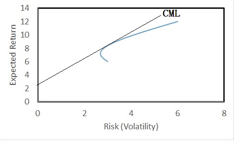
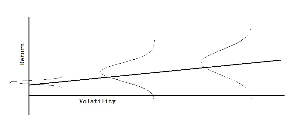
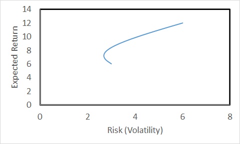
The relationship between risk and rewards, that reward increases with risk, is much engrossed in common knowledge. In investing, we have seen portfolio theory and capital market lines that confirm this notion.
But the risk-return line is far from straight. We have seen earlier that the X-axis (risk) in the case of an investment is the volatility of the portfolio. In the language of statistics, volatility is the standard deviation of the distribution. In other words, each point of the line represents a distribution (of returns), with higher and higher standard deviations from left to right.
While the expected returns, the mean of the distribution, are higher to the right, the chances of higher and lower returns (including losses) are also higher. The critical issue here is that no one knows the breadth of the distribution or its shape. Imagine if it is what Nassim Taleb calls a fat tail, an asymmetric distribution, or the occurrence of a heavy impact-low probability event.
We have seen how simple portfolio theory explains the relationship between risk and returns. For example, the representation below.
This leads to the development of what is known as the Capital Market Line (CML). CML is a concept that combines the risk-free asset and the market portfolio. It is the line connecting the risk-free return and tangent to the ‘efficient frontier’ of the portfolio.
The slope of the Capital Market Line (CML) is the Sharpe Ratio of the portfolio. Sharpe Ratio = (Return of the portfolio – risk-free rate) / Standard deviation
But there is something wrong with this line – or at least how people perceive the line of risk vs return. That is, next.
American economist and political commentator Thomas Sowell summarises the core of decision-making, like nobody has, in his famous quote: There Are No Solutions, Only Trade-offs.
A crucial thing in trade-off is the assessment of the consequence of each option. A common practice in investment decisions is the cost-benefit analysis.
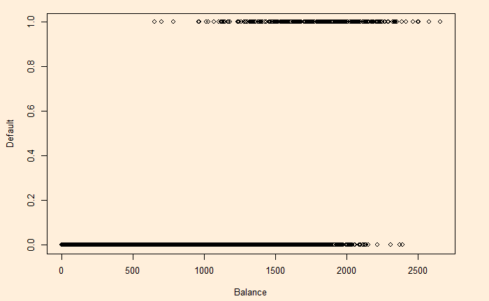
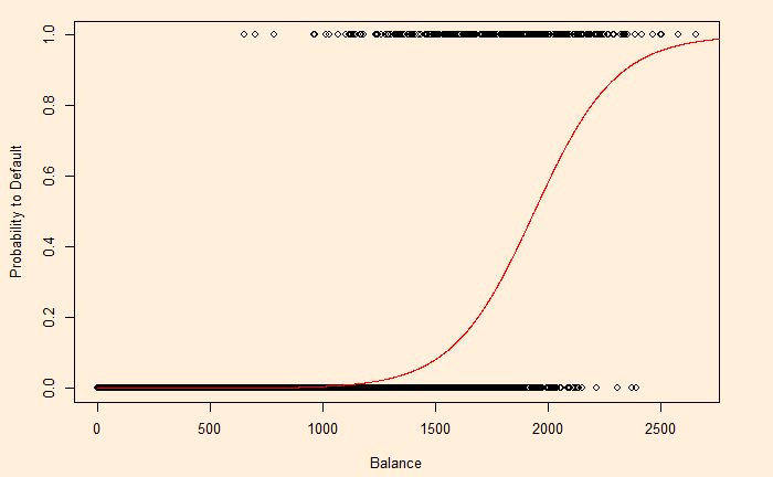
We have seen logistic regression as a means to estimate the probability of outcomes in classification problems where the response variable has two or more values. We use the ‘Default’ dataset from ‘ISLR2’ to illustrate. The data set contains 10000 observations on the following four variables:
default
: A factor with levels No and Yes indicating whether the customer defaulted on their debt

student:
 factor with levels No and Yes indicating whether the customer is a student

balance:
The average balance that the customer has remaining on their credit card after making their monthly payment

income: Income of customer
We change YES to 1 and NO to 0 and plot default vs balance.
Let p(X) be the probability that Y = 1 given X. The simple form that fits this behaviour is:
The beta values (the intercept and slope) are obtained by the ‘generalised linear model’, glm function in R.
D_Data <- Default
D_Data$def <- ifelse(D_Data$default=="Yes",1,0)
model <- glm(def ~ balance, family = binomial(link = "logit"), data = D_Data)
summary(model)
Call:
glm(formula = def ~ balance, family = binomial(link = "logit"),
    data = D_Data)

Deviance Residuals:
    Min       1Q   Median       3Q      Max
-2.2697  -0.1465  -0.0589  -0.0221   3.7589

Coefficients:
              Estimate Std. Error z value Pr(>|z|)
(Intercept) -1.065e+01  3.612e-01  -29.49   <2e-16 ***
balance      5.499e-03  2.204e-04   24.95   <2e-16 ***
---
Signif. codes:  0 ‘***’ 0.001 ‘**’ 0.01 ‘*’ 0.05 ‘.’ 0.1 ‘ ’ 1

(Dispersion parameter for binomial family taken to be 1)

    Null deviance: 2920.6  on 9999  degrees of freedom
Residual deviance: 1596.5  on 9998  degrees of freedom
AIC: 1600.5

Number of Fisher Scoring iterations: 8
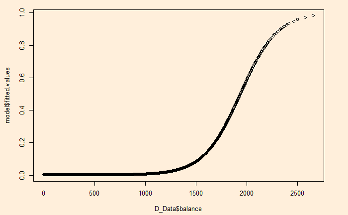
Now, we will test how good the model predictions are by plotting the function using the regressed beta0 ( = -10.65) and beta1 (= 0.0055).
plot(D_Data$balance, D_Data$def, xlab = "Balance", ylab = "Default")

y <- function(x){
  exp(-10.65+0.0055*x) / (1 + exp(-10.65+0.0055*x))
}

x <- seq(0, 3000)
lines(x, y(x), col = "red")
“The world’s human population is so large that the number of people alive today exceeds the number of people who died in the past!” Surely, you must have heard such claims. But how many of you have verified the truth behind such statements? Well, the Population Reference Bureau (PRB) do have estimates on it.
The number of people who ever lived is related to three factors:
The duration of human existence
The average number of people at different periods in history
The birth rate during each period.
The duration of human existence
The assumption was made based on the current evidence that modern Homo sapiens appeared around 190,000 B.C.E., originated in Africa.
The average number of people
Available information/estimations about the world populations in different eras of human history are collected.
YEAR
POPULATION
190,000 B.C.E
2
50,000 B.C.E.
2,000,000
8000 B.C.E.
5,000,000
1 C.E.
300,000,000
1200
450,000,000
1650
500,000,000
1900
1,656,000,000
2000
6,149,000,000
2022
7,963,500,000
Birth rate (BR)
Humans’ average life expectancy (LE) has stayed at about 12 years for most of history. Twelve years translates to 1000/12 ~ 80 births per year per 1,000 population. The number has since improved to the present value of 17. This equation (BR = 1000/LE) works in a stable population.
Once the birthrates are available at the different periods, one can assume a stable population between intervals and estimate the births each year (in between those intervals) as the number of years (between two periods) x BR x average population /1000
The estimated cumulative number of humans as of 2022 was 117,020,448,575. In other words, today’s world population of 7,963,500,000 (2022) is 6.8% of all homo sapiens ever lived.
Reference
How Many People Have Ever Lived on Earth?: prb.org
Anna, Bob and Claire are doing a three-way duel (a truel). Anna has an accuracy of 1/3, Bob has 2/3, and Claire is an excellent marksman with 1 (100%) accuracy. They must take turns shooting. Since each player knows others’ skills and all are rational, what would Anna do in the competition?
If Anna starts the duel and aims at Bob, there is a 1/3 chance she will shoot Bob. In that case, Claire has the next turn and will end Anna. On the other hand, if Anna aims at Claire, there is a 1/3 chance that Bob gets a chance to aim at Anna and end her with a 2/3 chance. So, it is clear that missing shots is a better option for Anna. So, she must shoot in the air first.
In the next chance, Bob will aim at the more prominent threat, i.e., Claire. Then there is a 2/3 chance of a showdown with Anna and a 1/3 chance that the showdown will be between Anna and Claire. Let P(A) be the probability that Anna survives, P(A, B) be the chance Alice wins the duel with Bob and P(A, C) Alice wins against Claire.
P(A) = 2/3 x P(A, B) + 1/3 x P(A, C) P(A) = 2/3 x 3/7 + 1/3 x 1/3 = 25/63