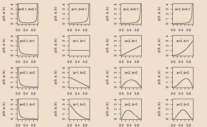
Bias in a Coin and Beta Prior

Bias in a Coin and Beta Prior Read More »
Bland-Altman analysis is used to study the agreement between two measurements. Here is how it is created.
Step 1: Collect the two measurements
Sample_Data <- data.frame(A=c(6, 5, 3, 5, 6, 6, 5, 4, 7, 8, 9,
10, 11, 13, 10, 4, 15, 8, 22, 5), B=c(5, 4, 3, 5, 5, 6, 8, 6, 4, 7, 7, 11, 13, 5, 10, 11, 14, 8, 9, 4))
Step 2: Calculate the means of the measurement 1 and measurement 2
Sample_Data$average <- rowMeans(Sample_Data) Step 3: Calculate the difference between measurement 1 and measurement 2
Sample_Data$difference <- Sample_Data$A - Sample_Data$BStep 4: Calculate the limits of the agreement based on the chosen confidence interval
mean_difference <- mean(Sample_Data$difference)
lower_limit <- mean_difference - 1.96*sd( Sample_Data$difference )
upper_limit <- mean_difference + 1.96*sd( Sample_Data$difference )
Step 5: Create a scatter plot with the mean on the X-axis and the difference on the Y-axis. Mark the limits and the mean of difference.
ggplot(Sample_Data, aes(x = average, y = difference)) +
  geom_point(size=3) +
  geom_hline(yintercept = mean_difference, color= "red", lwd=1.5) +
  geom_hline(yintercept = lower_limit, color = "green", lwd=1.5) +
  geom_hline(yintercept = upper_limit, color = "green", lwd=1.5) +
  ggtitle("")+
       ylab("Difference")+
xlab("Average") 
Following are the free throw statistics from basketball great Larry Bird’s two seasons.
Total pairs of throws: 338
Pairs where both throws missed: 5
Pairs where one missed: 82
Pairs where both made: 251
Test the hypothesis that Mr Bird’s free throw follows binomial distribution with p = 0.8.
H0 = Bird’s free throw probability of success followed a binomial distribution with p = 0.8
HA = The distribution did not follow a binomial distribution with p = 0.8
We will use chi-square Goodness of Fit to test the hypothesis. The probabilities of making 0, 1 and 2 free throws for a person with a probability of success of 0.8 is
bino_prob <- dbinom(0:2, 2, 0.8) 0.04 0.32 0.64The chi-square test is:
chisq.test(child_perHouse, p = bino_prob, rescale.p = TRUE)
	Chi-squared test for given probabilities

data:  child_perHouse
X-squared = 17.256, df = 2, p-value = 0.000179
Larry Bird and Binomial Distribution Read More »
‘This sentence is false’ is an example of what is known as the Liar Paradox.
This sentence is false.
Look at the first option for the answer—true. To do that, we check what the sentence says about itself. It says about itself that it is false. If it is true, then it is false, which is a contradiction, and therefore, the answer ‘true’ is not acceptable.
The second option is false. Since the sentence claims about itself as false, then it’s false that it’s false, which again is a contradiction.
This Sentence is False! Read More »
It has been found that the scores obtained by students follow a normal distribution with a mean of 75 and a standard deviation of 10. The top 10% end up in the university. What is the minimum mark for a student if she gets admission to the university?
The first step is to convert the percentage to the Z-score. It can be done in one of two ways.
qnorm(0.1, lower.tail = FALSE)qnorm(0.9, lower.tail = TRUE)1.28Note that if you do not specify, the default for qnorm will be lower.tail = TRUE.
Z = (X – mean)/standard deviation
X = Z x standard deviation + mean
X = 1.28 x 10 + 75 = 87.8
The Z-score and Percentile Read More »
We have seen how R calculates the chi-squared test for independence. This time, we will estimate it manually while developing an intuition of the calculations. Here are the observed values.
| High School | Bachelors | Masters | Ph.d. | Total | |
| Female | 60 | 54 | 46 | 41 | 201 |
| Male | 40 | 44 | 53 | 57 | 194 |
| Total | 100 | 98 | 99 | 98 | 395 |
Now, the expected values are estimated by assuming independence, which allows us to multiply the marginal probabilities to obtain the joint probabilities.
The observed frequency of the female and high school is 60. The expected frequency, if they are independent, is the product of the marginals (being a female and being in high school): (201/395) x (100/395) x 395. The last multiplication with 395 is to get the frequency from the probability. (201/395) x (100/395) x 395 = 50.88. In the same way, we can estimate the other cells.
| High School | Bachelors | Masters | Ph.d. | Total | |
| Female | 50.88 | 49.87 | 50.38 | 49.87 | 201 |
| Male | 49.11 | 48.13 | 48.62 | 48.13 | 194 |
| Total | 100 | 98 | 99 | 98 | 395 |
chi-squared = sum(observed - expected)2 / expected
= (60 - 50.88)2/50.88 + (54 - 49.87)2/49.87 + (46 - 50.38)2/50.38 + (41 - 49.87)2/49.87 + (40 - 49.11)2/49.11 + (44 - 48.13)2/48.13 + (53 - 48.62)2/48.62 + (58 - 48.13)2/48.13 8.008746You can look at the chi-squared table for 8.008746 with degrees of freedom = 3 for the p-value.
Test for Independence – Illustration Read More »
Three machines make parts in a factory. The following information about the production line is available.
Machine 1 makes 50% of the parts
Machine 2 makes 25% of the parts
Machine 3 makes 25% of the parts
5% of the parts by Machine 1 are defective
10% of the parts by Machine 2 are defective
12% of the parts by Machine 3 are defective
If a part is randomly selected, what is the probability that it is defective?
The solution goes to a fundamental rule of probability that relates total probability to marginal and conditional probabilities.
P(A) = P(A ∩ B1) + P(A ∩ B2) + … + P(A ∩ Bk)
P(A) = P(B1)P(A|B1) + P(B2)P(A|B2) + … + P(Bk)P(A|Bk)
Using this equation, we get
P(Defective) = P(Machine1)P(Defective|Machine1) + P(Machine2)P(Defective|Machine2) + P(Machine3)P(Defective|Machine3)
= 0.5×0.05 + 0.25×0.1 + 0.25×0.12 = 0.08 or 8% chance.
Law of Total Probability Read More »
Here is a step-by-step process for performing a chi-squared test of independence using R. The following is a survey result from a random sample of 395 people. The survey asked about participants’ education levels. Based on the collected data, do you find any relationships? Consider a 5% significance level.
| High School | Bachelors | Masters | Ph.d. | Total | |
| Female | 60 | 54 | 46 | 41 | 201 |
| Male | 40 | 44 | 53 | 57 | 194 |
| Total | 100 | 98 | 99 | 98 | 395 |
data= matrix(c(60, 54, 46, 41, 40, 44, 53, 57), ncol=4, byrow=TRUE)

colnames(data) = c('High School','Bachelors','Masters','Ph.d.')
rownames(data) <- c('Female','Male')

survey=as.table(data)
survey
High School Bachelors Masters Ph.d.
Female 60 54 46 41
Male 40 44 53 57chisq.test(survey) Pearson's Chi-squared test
data: survey
X-squared = 8.0061, df = 3, p-value = 0.04589The chi-squared = 8.0061 at degrees of freedom = 3. As the p-value = 0.04589 < 0.05, we reject the null hypothesis; the education level depends on the gender at a 5% significance level.
Chi-Square Tests: PennState
Gender and Education Level Read More »
A recent survey showed the number of children per household as follows:
| # Children per household | Population |
| 0 | 4.3 |
| 1 | 1.0 |
| 2 | 2.3 |
| 3 | 0.3 |
| 4 | 0.2 |
| 5 | 0 |
Check how the data compares with a Poisson distribution with lambda = 1.
You may recall that lambda is the expected value of Poisson distribution. First, we create the Poisson probabilities for each category from the number of children per household = 0.
poi_prob <- dpois(0:5, 1)0.367879441 0.367879441 0.183939721 0.061313240 0.015328310 0.003065662Having established the expected probabilities, we perform the chi-squared test.
poi_prob <- dpois(0:5, 1)
child_perHouse <- c(4.3, 1.0, 2.3, 0.3, 0.2, 0)
chisq.test(child_perHouse, p = poi_prob, rescale.p = TRUE)
Chi-squared test for given probabilities
data: child_perHouse
X-squared = 2.4883, df = 5, p-value = 0.7783Children and Poisson Distribution Read More »
We have seen family-wise error rate (FWER) as the probability of making at least one Type 1 error when conducting m hypothesis tests.
FWER = P(falsely reject at least one null hypothesis)
= 1 – P(do not reject any null hypothesis)
= 1 – P(∩j=1n {do not falsely reject H0,j})
If each of these tests is independent, the required probability equals (1 – α)n, and
FWER = 1 – (1 – α)n
For example, if the significance level is 0.05 (α) for five tests,
FWER = 1 – (1 – 0.05)5
And, if you make n = 100 independent tests,
FWER = 1 – (1 – 0.05)100 = 0.994; guaranteed to make at least one Type I error.
One of the classical methods of managing the FWER is the Bonferroni correction. As per this, the corrected alpha is the original alpha divided by the number of tests, n.
Bonferroni corrected α = original α / n
For five tests,
FWER = 1 – (1 – 0.05/5)5 = 0.049; and for 100 tests
FWER = 1 – (1 – 0.05/100)100 = 0.049
Family-Wise Error Rate and The Bonferroni Correction Read More »