All

1-Sample t-Test

We will do a 1-sample t-test from start to finish using R. You know about the t-test, and we have done it before.

What is a 1-sample t-test?

It is a statistical way of comparing the mean of a sample dataset with a reference value of the population. The reference value (reference mean) becomes the null hypothesis and what we do in the t-test is nothing but hypothesis testing.

Assumptions

There are a few key assumptions that we make before applying the test. First, it has to be a random sample. In other words, it has to be representative; otherwise, it would not provide any valid inference for the population. The second condition requires that the data must be continuous. Finally, the data should follow a normal distribution or have more than 20 observations.

Example

You have done a major revamp of the school curriculum this year. You know the state-level average test score last year was 50. You like to find out whether the average score this year is different from the previous. So, you conducted a random sample of 20 participants, and their scores are below:

StudentScore
140.5
250.1
360.2
451.3
542.1
657.2
737.9
847.2
958.3
1060
1161.2
1252.5
1366
1455
1558
1655.1
1747.4
1852.1
1963.1
2052.1
mean = 53.365

Is that significant?

The mean = 53.365 suggests there was an improvement in students’ scores. But that is a quick conclusion; after all, we took only a sample, which will have variability, and, unlike the population mean, the sample means will follow a distribution. So we will do testing the following hypotheses:

The null hypothesis, N0: The mean of the population this year is 50
The alternative hypothesis, NA: The mean of the population this year is not 50
But, before that, let’s plot the data. It is a good habit that can already give a feel of the data quality, scatter, outliers etc.

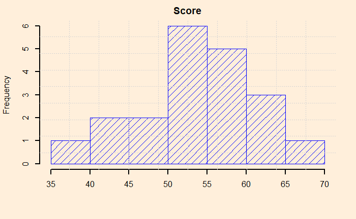
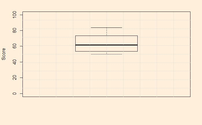
The data look pretty ok, with no outliers, reasonably distributed etc. Now, the t-test. It’s simple: use the R function, t.test (stats package), and you get everything.

test_data <- data.frame(score = c(40.5,50.1,60.2, 51.3, 42.1, 57.2, 37.9, 47.2, 58.3, 60, 61.2, 52.5, 66, 55, 58, 55.1, 47.4, 52.1, 63.1, 52.1))
t.test(test_data$score, mu = 50)

The output is as follows

	One Sample t-test

data:  test_data$score
t = 1.9807, df = 19, p-value = 0.06229
alternative hypothesis: true mean is not equal to 50
95 percent confidence interval:
 49.80912 56.92088
sample estimates:
mean of x 
   53.365 

We shall see the inferences of this analysis in the next post.

1-Sample t-Test Read More »

Ecological Fallacy – What Radelet Saw

Michael Radelet’s study in 1981 is an example of ecological fallacy but, more importantly, exposed the racial disparity that existed in the process of ensuring criminal justice in the US.

Radelet collected data from 20 counties of Florida indictments of murders that occurred in 1976 and 1977. His research team have identified 788 homicide cases, and after cleanup of incomplete information, 637 remained for further investigation.

Ecology

Let us start with the overall results: the race composition of the death penalty is 5.1% (17 death penalties out of a total of 335 defendants) for blacks and 7.3% (22 out of 302). There is nothing much in it, or if you are right-leaning with a bit of vested interest, you might even say the judges are more likely to hand death penalties to the whites!

The details

Now, what happens to justice if the victims were white? If the person died in the case was white, there is a 16.7% chance for the black defendants to get a death sentence vs 7.7% for a white. On the other hand, if the person murdered was back, the percentages are 2.2 for blacks and 0 for whites. Black lives were priced lower, and whites seemed to have some birth rights to take out some of it!

The complete dataset is below; you may do the math yourself.

# CasesFirst degree
indictments
Sentenced
to Death
Non-Primary
White victim
Black defendant635811
White defendant15112419
Non-Primary
Black victim
Black defendant103566
White defendant940
Primary
White victim
Black defendant310
White defendant134733
Primary
Black victim
Black defendant166510
White defendant840
Total63737139

Radelet, M.L.; Racial Characteristics and the Imposition of the Death Penalty, American Sociological Review, 1981, 46 (6), 918-927

Ecological Fallacy – What Radelet Saw Read More »

Ecological fallacy

A lot of data we know describe the general trends of a region or group than from its members. E.g. the crime rate of a city is estimated based on the total number of crimes divided by the number of people. It is not calculated based on surveys of every individual member. A city can be high in crime rates, yet 99% of the individuals are not under any threat to their life or property. In other words, there may be a few pockets in the city that experience disproportionately more crimes than the rest.

Ecological fallacy describes the logical error when we take a statistic meant to represent an area or group and apply it to the individuals or objects inside. It gets the name because the data was meant to describe the system, the environment or the ecology.

A lot of stereotypes arise out of ecological fallacy. A well-known example is racial profiling, in which a person is discriminated against or stereotyped against her ethnicity, religion or nationality. Simpson’s paradox, something we had discussed in the past, is a special case of ecological fallacy.

A classical case was the 1950 paper published by Robinson in American Sociological Review. He found a positive correlation between migrants (colour) and illiteracy. Yet, he found, at the state level, a negative correlation (-0.53) between illiteracy and the number of people born outside the US. This was counterintuitive. One possible explanation is that while migrants tend to be more illiterate, they tend to migrate to regions that are, on average, more literate, such as big cities.

Robinson, W. S; American Sociological Review, 1950, 15 (3),  351-357.

Ecological fallacy Read More »

p-value Fallacy

We have seen the p-value before. A higher p-value of a test suggests that the sample results are consistent with the null hypothesis. Correspondingly, to reject the null hypothesis, you like to have lower p-values.

p-values are probabilities observing this extreme sample statistics when the null hypothesis is correct. For example, if 0.05 is the p-value of a study to test the effectiveness of a drug, then you should understand that even if the medicine has no effect, 5% of the studies will give the results you obtained.

It doesn’t stop here. People now think that 5% is the error rate of the test. And this is termed the p-value fallacy. The error associated with a particular p-value is estimated to be much higher than the p-value.

p-value Fallacy Read More »

Counting Cards

Blackjack is a special kind of casino game as it doesn’t have independence from hand to hand. Because a card, once left the deck, can not come back until the deck is reshuffled. It means that the previous card affects the probability of the next card, and therefore, card counting is a possible means to estimate future win potential. Consider this:

The probability of drawing a natural from a deck is

P(\text{Natural}) = 2*\frac{4}{52}*\frac{16}{51} \approx 0.0483 \approx \frac{1}{21}

Suppose an ace is removed from the deck. The updated probability for the natural is:

P(\text{Natural}) = 2*\frac{3}{51}*\frac{16}{50} \approx 0.0376 \approx \frac{1}{27}

Or if a three was removed,

P(\text{Natural}) = 2*\frac{4}{51}*\frac{16}{50} \approx 0.0502 \approx \frac{1}{20}

Counting Cards Read More »

The Blackjack

What is the probability of getting a natural or blackjack when a player delt two-card total of 21 from a well-shuffled 5-deck shoe?

casino, poker, blackjack-5619014.jpg

Getting exactly 21 from two cards means you must get an ace (ace can take 1 or 11 at the player’s discretion) and a ten-count card (number 10 or a face card). We will estimate the probability by two different methods.

Method 1

From cards from n-decks, the probability of getting an ace in the first deal followed by a 10 in the second is given by:

\frac{4n}{52n}*\frac{16n}{52n-1}

Similarly, the probability of having a 10-card followed by an ace is:

\frac{16n}{52n}*\frac{4n}{52n-1}

Combining the two, you get the total probability of natural.

P(\text{Natural}) = \frac{4n}{52n}*\frac{16n}{52n-1} + \frac{16n}{52n}*\frac{4n}{52n-1} = \frac{32n}{13(52n-1)}

For a 5-deck shoe, substitute n = 5, and you get 0.0475 or 4.75%.

Method 2

We will use the familiar combinations formula to get the same.

P(\text{Natural}) = \frac{_{4n}C_1*_{16n}C_1}{_{52n}C_2} = \frac{20*80}{33670} = 0.04752 (\text{ for n = 5})

Combinations Calculator

The Blackjack Read More »

Card Games – Continued

Five cards are dealt from a standard 52-card deck. What is the probability of drawing four face cards and an Ace? First, we do it analytically.

Combinations

We are choosing four face cards from the total possible 12 (and without replacement). Since the order of the deal doesn’t matter, it is a combination problem of the following form.

\\ _{12}C_4 = \frac{12!}{(12-4)!4!} = \frac{12!}{8!4!} \\ \\ = \frac{12*11*10*9}{4*3*2*1} = 495

Now, calculate the ways of choosing one ace card from a total of four.

\\ _{4}C_1 = \frac{4!}{(4-1)!1!} = \frac{4!}{3!} = 4

To get the required probability, we have to divide the product of the two with all the possible combinations (of selecting five cards from the deck of 52).

\\ _{52}C_5 = \frac{52!}{(52-5)!5!} = \frac{52!}{47!5!}  \\ \\ = \frac{52*51*50*49*48}{5*4*3*2*1} = 2598960

Finally, the probability is calculated by dividing the combination of getting four face cards and one ace card with the possibility of getting five cards from the deck.

\\ P = \frac{_{12}C_4 * _4C_1} {_{52}C_5} \\ \\ P = \frac{\frac{12!}{8!4!}*\frac{4!}{3!1!}}{\frac{52!}{47!5!}} \\ \\ \frac{495 * 4}{2598960} = 0.0007618432

We can execute the whole calculation using the following R code:

choose(12,4)*choose(4,1)/choose(52,5)

Monte Carlo

Let’s start building the deck as we did last time.

suits <- c("Diamonds", "Spades", "Hearts", "Clubs")
face <- c("Jack", "Queen", "King")
numb <- c("Deuce", "Three", "Four", "Five", "Six", "Seven", "Eight", "Nine", "Ten")

face_card <- expand.grid(Face = face, Suit = suits)
face_card <- paste(face_card$Face, face_card$Suit)

numb_card <- expand.grid(Numb = numb, Suit = suits)
numb_card <- paste(numb_card$Numb, numb_card$Suit)

Aces <- paste("Ace", suits) 

deck <- c(Aces, numb_card, face_card)

Now start drawing five cards at random and check your hands. Repeat that a million times, and count the number of times you got what you wanted. And divide it by the million.

B <- 1000000

results <- replicate(B, {

hand <- sample(1:52, 5, replace = FALSE)
deal <- deck[hand]

match_1 <- sum(face_card %in% deal)
match_2 <- sum(Aces %in% deal)

if(match_1 == 4 & match_2 ==1) {
  counter <- 1 
}else{
  counter <- 0
}
  
})

sum(results) / B 

Card Games – Continued Read More »

Card Games

Let’s play some card games. Today we will create a deck of cards using R programming.

There are 52 cards in a deck. And they fall into four suits – Diamonds, Spades, Hearts and Clubs. Each of these suits can have nine numbers (2 – 10), three faces (Jack, Queen and King) or an Ace. For example, a card can be an Ace of Clubs, another may be a four of Hearts etc.

suits <- c("Diamonds", "Spades", "Hearts", "Clubs")
numbers <- c("Ace", "Deuce", "Three", "Four", "Five", "Six", "Seven", "Eight", "Nine", "Ten", "Jack", "Queen", "King")

We will use the expand.grid function in R to create a data frame with all combinations of suits and numbers.

deck <- expand.grid(Number = numbers, Suit = suits)

If you print the output from the previous command (as_tibble(deck)), you get the following data frame with 52 rows. The top five rows are shown below.

Number
<fctr>
Suit
<fctr>
AceDiamonds
DeuceDiamonds
ThreeDiamonds
FourDiamonds
FiveDiamonds

It still doesn’t look like cards, as they are separated by the columns of the data frame. So we will paste them into each other and create one deck of 52 entries, as follows.

deck <- paste(deck$Number, deck$Suit)
“Ace Diamonds” “Deuce Diamonds” “Three Diamonds” “Four Diamonds” “Five Diamonds” “Six Diamonds” “Seven Diamonds” “Eight Diamonds” “Nine Diamonds” “Ten Diamonds” “Jack Diamonds” “Queen Diamonds” “King Diamonds” “Ace Spades” “Deuce Spades” “Three Spades” “Four Spades” “Five Spades” “Six Spades” “Seven Spades” “Eight Spades” “Nine Spades” “Ten Spades” “Jack Spades” “Queen Spades” “King Spades” “Ace Hearts” “Deuce Hearts” “Three Hearts” “Four Hearts” “Five Hearts” “Six Hearts” “Seven Hearts” “Eight Hearts” “Nine Hearts” “Ten Hearts” “Jack Hearts” “Queen Hearts” “King Hearts” “Ace Clubs” “Deuce Clubs” “Three Clubs” “Four Clubs” “Five Clubs” “Six Clubs” “Seven Clubs” “Eight Clubs” “Nine Clubs” “Ten Clubs” “Jack Clubs” “Queen Clubs” “King Clubs”

We will do the first two estimations now. How many kings are in the deck, and what is the probability of drawing a king from the deck?

kings <- paste("King", suits) 
deck %in% kings
sum(deck %in% kings) # output is 4
mean(deck %in% kings) # output is 0.07692308


# paste("King", suits) creates all kings (output:  "King Diamonds" "King Spades"   "King Hearts"   "King Clubs" )
# The command, %in%, searches for 'kings' inside the vector 'deck' and returns TRUE or FALSE, depending on whether it matched or not. 
# sum adds up all - each TRUE gets 1, and FALSE gets 0.
# mean gives the average: sum/total count

Card Games Read More »

Permutations and Combinations Continued

Five strong contenders are running a race. How many ways can the gold, silver and bronze be awarded? We have five possible athletes to choose from but three at a time. The order does matter here as these are first, second and third places. Also, one person can not be first and second, or repetition is not allowed. So it is a permutation problem.

\\ _nP_r = \frac{n!}{(n-r)!}  \\ _5P_3 = \frac{5!}{(5-3)!} = \frac{5!}{2!} = \frac{5 * 4 * 3 * 2 * 1}{2 * 1} = 60

Now, you have five topping choices to make pizza with three toppings. How many distinct pizzas can you make? The first thing to notice here is the lack of order – your selection of pepperoni, onions and mushrooms is no different from onions, pepperoni and mushrooms or mushrooms, onions, pepperoni etc. It becomes a combination problem.

\\ _nC_r = \frac{n!}{(n-r)! r!} \\ _{5}C_3 = \frac{5!}{(5-3)!3!} = \frac{5!}{2!3!} = \frac{5*4*3*2*1}{(2*1)((3*2*1)} = \frac{5*4}{2} = 10

Not to forget that this problem does not allow you to choose one-topping twice, which real shops may permit!

Permutations and Combinations Continued Read More »

Permutations and Combinations

At a party of 25 people, how many handshakes are expected if each person asks hands with every other? Is this a permutation problem or a combination?

Before that, what is a permutation, and what is a combination? They both represent different ways of arranging things from an available list of options. For example, how many unique passcodes are possible for a combination lock of 4 wheels? Let’s count. There are ten possibilities for the first wheel (0-9), another 10 for the second, and the same for the third and fourth. Total possibilities = 10 x 10 x 10 x 10 = 104 = 10000. Some people will say there are 9999 ways, as one is always available to start!

Permutations

How many four-digit numbers can you make from 4, 6, 7 and 8? It is different from the combination lock problem as you can’t get to use it again once you use up one of the digits. So let’s do the counting: in the first place, you have four possibilities; in the second place, since one of them is used up, you have three, then two and finally, the remaining one. So the total permutatoins are 4 x 3 x 2 x 1 = 24.

Permutations of n available options taken r at a time = nPr. In the digit case, it was 4P4

\\ _nP_r = \frac{n!}{(n-r)!} \\ \\ _4P_4 = \frac{4!}{(4-4)!} = \frac{4!}{0!} = \frac{4 * 3 * 2 * 1}{1} = 24

Combinations

The combination is where you make arrangements when the order does not matter. The handshake problem is a combination case. When two people shake their hands, one handshake happens. In other words, this becomes a permutation problem but discounting the double-counting. It is called combinations or nCr.

\\ _nC_r = \frac{n!}{(n-r)! r!} \\ \\ _{25}C_2 = \frac{25!}{(25-2)!2!} = \frac{25!}{23!2!} = \frac{25*24*23*22*....*1}{(23*22*21*....*1)((2*1)} = \frac{25*24}{2} = 300

300 unique handshakes will happen.

Factorial Calculator

Permutations and Combinations Read More »