All

Braess’s Paradox

Another counterintuitive experience similar to Downs–Thomson’s is Braess’s Paradox. As per this phenomenon, adding more roads to an existing network can slow down the overall traffic. Similar to the previous, we will see the mathematical explanation first.

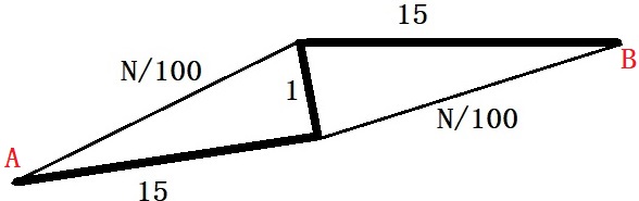
Suppose there are two routes to city B from city A, as shown in the picture – the top and bottom roads. The first part is narrow on the top road, followed by a broad highway. The situation is the opposite for the bottom road.

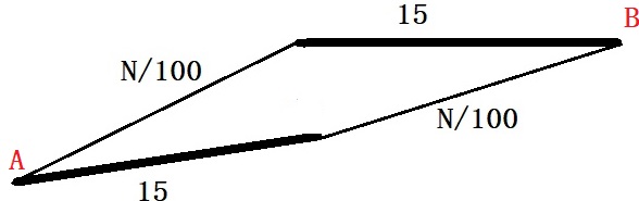
The highways are not impacted by the number of cars, whereas, for the narrower roads, the traffic time is related to the number of vehicles on the road – N/100, where N is the number of cars.

If there are 1000 cars in the city, the system will reach the Nash equilibrium by cars getting equally divided (in the longer term), i.e., 500 on each road. Therefore, each car to take
500/100 + 15 = 20 mins

Imagine a new interconnection built by the city to reduce traffic congestion. The travel time on the connection section is 1 minute. Let’s look at all scenarios.

Scenario 1: A car starts from the bottom highway, takes the connection, and moves to the top highway. Total time = 15 + 1 + 15 = 31 mins.
Scenario 2: One car starts from the top road, takes the connection, and moves to the bottom road, while the others follow the old path (not using the connection). Total time = 50/100 + 1 + 51/100 ~ 11 mins.

Scenario 2 seems a no-brainer to the car driver. But this news invariably reaches everyone, and soon, everyone starts taking the narrow paths! In other words, the narrow route is the dominant strategy. The total travel time now becomes:
1000/100 + 1 + 1000/100 = 21 min. This is more than the old state, a situation with no connection possible.

So, the condition without the connection road (or closing down the connection road) seems a better choice. And this is Braess’s paradox suggesting that a more complex system may not necessarily be a better choice.

Braess’s Paradox Read More »

Downs–Thomson paradox

Here is a game theory puzzle for you. The government proposes to build a highway between the two cities, A and B, that reduces the burden of the existing freeway. Here is the rationale behind the proposal.

There are two modes of arriving from A to B: 1) take the train, which takes 20 minutes, or 2) take the freeway using a car, which takes (10 + n/5) minutes, where n is the total number of cars on the road. Since the train is a public transit, it doesn’t matter how many people take it – it always takes 20 minutes to reach the destination. But if the new highway operates, the travel time becomes (5 + n/5) minutes. Note that the old freeway stops functioning once the new road is available.

What is your view on building the highway as a solution to reduce travel time, or are there alternate ideas to meet the objective?

The existing case

Suppose there are 100 commuters. Each can take the train and reach B in 20 minutes. That gives a few people the advantage of taking cars and reaching their destination earlier – until the travel time matches the following way.
20 = 10 + n/5
n = 50
Beyond 50 commuters, car travel will take longer than the train; therefore, 50 is an equilibrium number in the longer term.

The new case

The new equilibrium is estimated as follows:
20 = 5 + n/5
n = 75
In other words, more people will take the new route, but the travel time remains the same.

The paradox

This is a simplified game-theory explanation of what is known as the Downs–Thomson paradox. It says that comparable public transport journeys or the next best alternative defines the equilibrium speed of car traffic on the road.

Alternatives

On the other hand, if modifications are possible to reduce the commute time of the train, then overall travel time (for both railways and roads) can be reduced.

References

Downs–Thomson paradox: Wiki

The Problem with Faster Highways: William Spaniel

Downs–Thomson paradox Read More »

The Auction Game

Amy and Becky are in an auction for a painting. The rules of the auction are:

  1. Bidders must submit one secret bid.
  2. The minimum amount to bid is $10 and can be done in increments of $10
  3. Whoever bids the highest wins and will be charged an amount equal to the bid amount.
  4. In the event of a tie, the auction house will choose a winner based on a lot with equal probabilities.

Amy thinks the fair value of the painting is $56, and Becky thinks it’s $52. These valuations are also known to both. What should be the optimal bid?

The payoff matrix is:

Becky
Bid $40Bid $50
AmyBid $408, 60, 2
Bid $506, 03, 1

If Amy bids $40 and Becky $50, Becky wins the painting and her payoff is the value she attributes (52) – the payment (50)= $2. The loser wins or loses nothing.
If Amy bids $50 and Becky $40, Amy gets it, and her payoff will be the value (56) – what she pays (50) = $6.
If both bid at $40, Amy can get a net gain of 16 (56 – 40) at a probability of 0.5. That implies the payoff for Amy = $8. For Becky, it’s $12 x 0.5 = $6.
If both bid for $50, Amy’s payoff = $6 x 0.5 = $3 and Becky’s = $2 x 0.5 = $1

At first glance, it seems obvious that the equilibrium is where both are bidding for $40. If Amy thinks Becky will bid $40, Amy’s best response is to bid the same as her payoff is $8. The same is the case for Becky.
But if Amy expects Becky to go for $50, then Amy must also bid $50. Becky will also go along the same logic.

The Auction Game Read More »

Drunken Man Continues

The person in our previous two posts drinks every other day. As we have seen before, when he comes back, he must use the house key from the bunch of ten similar ones. As he can’t find which key is correct, he tries them individually when sober. When drunk, he pushes the same way but can’t distinguish which keys he has tried before.

What is the probability that he was inebriated on the day he unlocked the door on his seventh attempt?

It is a conditional probability problem, and the ask is:
The probability that he is drunk, given he got the right key on the seventh attempt or P(D|7). We can use Bayes’ rule, that is,

P(D|7) = \frac{P(7|D)*P(D)}{P(7|D)*P(D) + P(7|S)*P(S)}

The terms are:
P(7|D) – Probability he opens on his 7th try, given he is drunk
P(D) – Prior probability that he is drunk on the day
P(7|S) – Probability he opens on his 7th try, given he is sobber
P(S) – Prior probability that he is sobber on the day

P(7|D) = (9/10)6 x (1/10) = 0.053
P(7|S) = (9/10)x(8/9)x(7/8)x(6/7)x(5/6)x(4/5)x(1/4) = 1/10 = 0.1
P(D) = 1/2
P(S) = 1/2

P(D|7) = \frac{0.053 * 0.5}{0.053 * 0.5 + 0.1 * 0.5} = 0.35

There is a 35% probability that he is drunk.

Drunken Man Continues Read More »

Drunken Man and the Room Key – Simulations

Here is the simulation of the problem of the drunken man and keys. Let me repeat the problem statement: A drunk man reaches his home and tries the door key from a bunch of 10 keys. If the first key doesn’t work, he returns the key to the bunch and randomly selects another key repeatedly until he opens the door. The question is: which precise trial has the highest probability of opening the door?

library(reshape)
library(ggplot2)

key <- 3
itr <- 100000

drunk <- replicate(itr, {
index <- 1
    for(i in 1:100) {
    sel <- sample(seq(1:10), 1, replace = TRUE, prob = rep(1/10,10))  
if(sel == key){
 index 
 break 
}else{
  index = index + 1
}
    }
index
    })

temp.melt <- melt(table(drunk))

ggplot(temp.melt, aes(x = drunk, y = value/itr)) +
  theme_bw() +
  geom_bar(stat = "identity", fill = "brown") +
  xlim(0,20) +
 
labs(x= "Attempt #",
       y= "Probability") +
  theme(legend.position="none") +

theme(text = element_text(color = "black"), 
        panel.background = element_rect(fill = "antiquewhite1"), 
        plot.background = element_rect(fill = "antiquewhite1"),
        panel.grid = element_blank())

Drunken Man and the Room Key – Simulations Read More »

Drunken Man and the Room Key

Here is an interesting but misleading probability question: A drunk man reaches his home and tries the door key from a bunch of 10 keys. If the first key doesn’t work, he returns the key to the bunch and randomly selects another key repeatedly until he opens the door. The question is: which precise trial has the highest probability of opening the door?

The question is misleading because it does not ask you to guess by which try the person will find the right key and open the door. We’ll come to that topic a little later. The task is to find the probability of finding the right key at each try and show which one is the highest.

The probability of finding the right key in his first attempt = 1/10; ten keys and finding one at random is one out of 10 possible options.
The probability of finding the right key in his second attempt = (9/10)x(1/10); it is the joint probability of not getting the right key in the first attempt (9/10) AND the chance of hitting the right on the second try.
The probability of finding the right key in his third attempt = (9/10)x(9/10)x(1/10). Here is the summary:

AttemptProbability
10.1
20.09
30.081
40.0729
50.06561

It doesn’t mean that person will open the door in the first attempt or never. We need to estimate something different to find how the probability of opening the door changes with attempts. The chance he opened the door in his second attempt is:
Probability he opened in the first OR probability he opened in the second = 1/10 + (9/10)*(1/10). Here is how that develops.

AttemptProbabilityProbability of
Right key by
Attempt
10.10.1
20.090.19
30.0810.27
40.07290.34
50.065610.41
60.0590.47

There is about a 50% chance he will open the door by his sixth attempt.

Drunken Man and the Room Key Read More »

Hide and Seek with Camouflage

Here is another hide-and-seek game but played with an inverse handicap. If the last case would have given a clue to the seeker 75% of the time, this time, it would help the hider 75% of the time on one location, i.e., the house. So the situation is

  1. There are two options to hide – behind bushes, behind the house.
  2. If the person hides behind the house, and the opponent searches the house, there is a 75% chance the seeker will not spot the hider (camouflage effective 75% of the time.
  3. If the person hides behind the bush, and the opponent searches it, it is normal, and no camouflage works.

We have seen similar puzzles before. Suppose there was no complication of camouflage; the players should mix their choices randomly at equal probabilities (0.5).

How should one search?

Let p be the probability that the seeker should search behind the house. The best value for p is such a way that the hider finds no particular incentive to choose one place over the other. In other words, the p makes the payoffs for the hider to hide behind bush and house equal.

Payoff to hide behind house = Payoff to hide behind bushes.
Pay off for hide behind house = p[1 x 0.75 + 0 x 0.25] + (1-p) x 1 = 0.75p + 1 – p
Pay off for hiding behind bushes = p x 1 + (1-p) x 0 = p

If the hider hides behind the house and the seeker searches the house, there is a 75% probability that she will gain one point and a 25% chance of zero. On the other hand, if the hider is behind the house and the seeker searches the bush, the hider gets a full score (one).

Solving for p,
0.75p + 1 – p = p
p = 0.8

How should one hide?

Let q be the probability that the hider must hide behind the house. Following the logic as before,

Payoff to search behind house = Payoff to search behind bushes.
Payoff to search behind house = q[0 x 0.75 + 1 x 0.25] + (1-q) x 0 = 0.25q
Payoff to search behind bushes = q x 0 + (1-q) x 1 = 1 – q

Solving for q,
0.25q = 1 – q
q = 0.8

Reference

Camouflaged Hide and Seek: William Spaniel

Hide and Seek with Camouflage Read More »

Hide and Seek Continued

We have seen a counterintuitive solution to the particular hide-and-seek game in which a signal (light) comes up at a fixed probability from one of the locations should one choose to hide there. Here is how one should hide, given the chance of the signal from the very location.

Let’s develop some intuition over the message from the plot. When there is no signal from one of the locations (the house), it becomes a normal hide-and-seek, and the person who hides must choose both places randomly at a 50:50 chance. On the other hand, when there is a signal from the house, the seeker can use it to her advantage, as some of the uncertainty over hiding behind the house gets eliminated by the presence of a signal and can search the other place more often. Once you understand the seeker’s mind, the hider must choose the house more often to counter the opponent.

The extreme case is when the probability of the signal is 99.99%, where the seeker can almost ignore the house and concentrate on the bushes. And that’s what the seeker will do, as seen in the plot below.

Hide and Seek Continued Read More »

Hide and Seek of the Second Order

Annie and Becky are playing hide and seek. Annie wants to hide, and it’s Becky’s job to find out. Annie has two choices – hide behind a house or the bushes. But there is a problem: if she hides behind the hose, there is a 75% probability that the surveillance system will catch her and a light will lit in the front. How often should Annie try to hide behind the house?

We have seen similar puzzles before. Suppose there was no complication due to light. In that case, intuition suggests that Annie and Becky should mix their choices randomly at equal probabilities.

Probabilities for searching

Becky’s strategy is designed to make both choices equally attractive to Annie. Let p be the probability that Becky search the house. Then, for Annie, the payoffs much match.

Hide behind house = Hide behind bushes.
Pay off for hide behind house = 0 x 0.75 + 0.25 [0 x p + 1 x (1-p)].
Pay off for hiding behind bushes = 1 x p + 0 x (1-p)

Explanation for the first equation. If Annie hides behind the house, there is a 75% probability that the light will lit and Becky will go and find her (or Annie ends up with 0). On the other hand, inside the 25% case, where no light is lit, there is a p chance Becky will go for the house and a (1-p) chance Becky will miss.

Solving for p,
0.25 – 0.25 p = p
p = 0.2

Probabilities for hiding

Let q be the probability for Annie to hide behind the house. Note that Becky will need to apply probabilities only when there is no light in front of the house. Annie’s strategy is to make payoffs for Becky equal (given no light).

The chance that Annie hides behind the house given no light is a conditional probability, and we must apply Bayes’ rule.

P(HH|NL) = P(NL|HH) x P(HH) / [ P(NL|HH) x P(HH) + P(NL|HB) x P(HB)]
= 0.25q /[0.25q + (1-q)]

Similarly, The probability Annie hides behind the bushes given no light is:
P(HB|NL) = P(NL|HB) x P(HB) / [P(NL|HB) x P(HB) + P(NL|HH) x P(HH)]
= (1-q) /[(1-q) + 0.25q]

Now, back to payoffs:

Payoff for Search house | no light = Payoff for Seach bushes | no light
Payoff for Search house | no light = 1 x [0.25q /[0.25q + (1-q)]] + 0 x (1-q) /[(1-q) + 0.25q]
Payoff for Search bushes | no light = 0 x [0.25q /[0.25q + (1-q)]] + 1 x (1-q) /[(1-q) + 0.25q]

0.25 q /[0.25q + (1-q)]] = (1-q) /[(1-q) + 0.25q]
0.25 q = (1-q)
q = 1/1.25 = 0.8

This is counterintuitive; Annie will hide behind the house 80% of the time, knowing the light will be lit 75% of those occasions.

Reference

Expert-Level Hide and Seek: William Spaniel

Hide and Seek of the Second Order Read More »

Banzhaf Power Index – Continued

The calculation of the Banzhaf Power Index is as follows.

  1. List all winning coalitions
  2. In each collision, identify the critical players
  3. Count how many times each player is critical
  4. Convert these counts to fractions by dividing them by how many times any player is critical.

Here are a few definitions before we go further:

  1. A coalition is a group of players voting the same way
  2. Winning coalition: If the total weight of the coalition is equal to or greater than the quota, it is a winning coalition.
  3. Critical player: If by leaving the coalition, a player in a coalition makes a winning coalition into a losing one.

All coalitions

Following are all the three-player combinations

PP <- c(15, 25, 10, 30, 20)

PP_Comb <- combinations(n = 5, r = 3, v = PP, set = FALSE)
P2_Comb <- as.data.frame(PP_Comb) 
P2_Comb$Sum <- rowSums(PP_Comb) 
PlayerPlayerPlayerTotal WeightWinning
Coalition
15251050NO
15253070YES
15252060YES
15103055YES
15102045NO
15302065YES
25103065YES
25102055YES
25302075YES
10302060YES

All four-player combinations

PP <- c(15, 25, 10, 30, 20)

PP_Comb <- combinations(n = 5, r = 4, v = PP, set = FALSE)
P2_Comb <- as.data.frame(PP_Comb) 
P2_Comb$Sum <- rowSums(PP_Comb) 
PlayerPlayerPlayerPlayerTotal WeightWinning
Coalition
1525103080YES
1525102070YES
1525302090YES
1510302075YES
2510302085YES

Finally, the 5-player combination: 15, 25, 10, 30, 20 = 100

The table of all the winning coalitions with critical players in bold follows.

P2,P4 (25,30)
P1, P2, P4 (15, 25, 30)
P1, P2, P5 (15, 25, 20)
P1, P3, P4 (15, 10, 30)
P1, P4, P5 (15, 30, 20)
P2, P3, P4 (25, 10, 30)
P2, P3, P5 (25, 10, 20)
P2, P4, P5 (25, 30, 20)
P3, P4, P5 (10, 30, 20)
P1, P2, P3, P4 (15, 25, 10, 30)
P1, P2, P3, P5 (15, 25, 10, 20)
P1, P2, P4, P5 (15, 25, 30, 20)
P1, P3, P4, P5 (15, 10, 30, 20)
P2, P3, P4, P5 (25, 10, 30, 20)
P1, P2, P3, P4, P5 (15, 25, 10, 30, 20)
PlayerCritical
Times
Banzhaf
Power Index
P133/26
=11.5%
P277/26
= 26.9%
P322/26
= 7.7%
P499/26
= 42.3%
P555/26
= 19.2%
Total26

Player 4 has the highest voting power, with Banzhaf Power Index = 42.3%.

Banzhaf Power Index – Continued Read More »