All

The Capital Market Line: Illusion of Return

The relationship between risk and rewards, that reward increases with risk, is much engrossed in common knowledge. In investing, we have seen portfolio theory and capital market lines that confirm this notion.

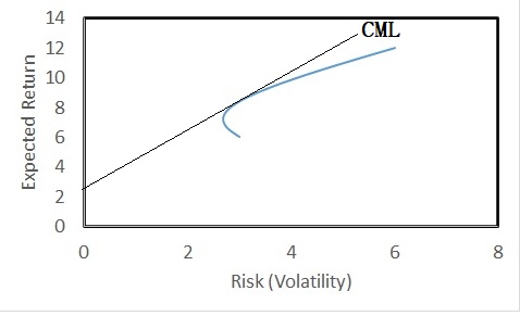
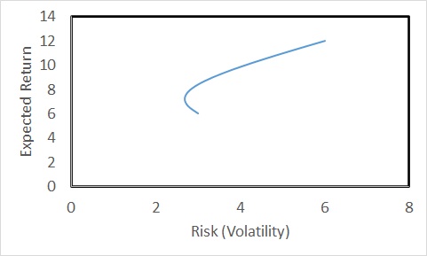
But the risk-return line is far from straight. We have seen earlier that the X-axis (risk) in the case of an investment is the volatility of the portfolio. In the language of statistics, volatility is the standard deviation of the distribution. In other words, each point of the line represents a distribution (of returns), with higher and higher standard deviations from left to right.

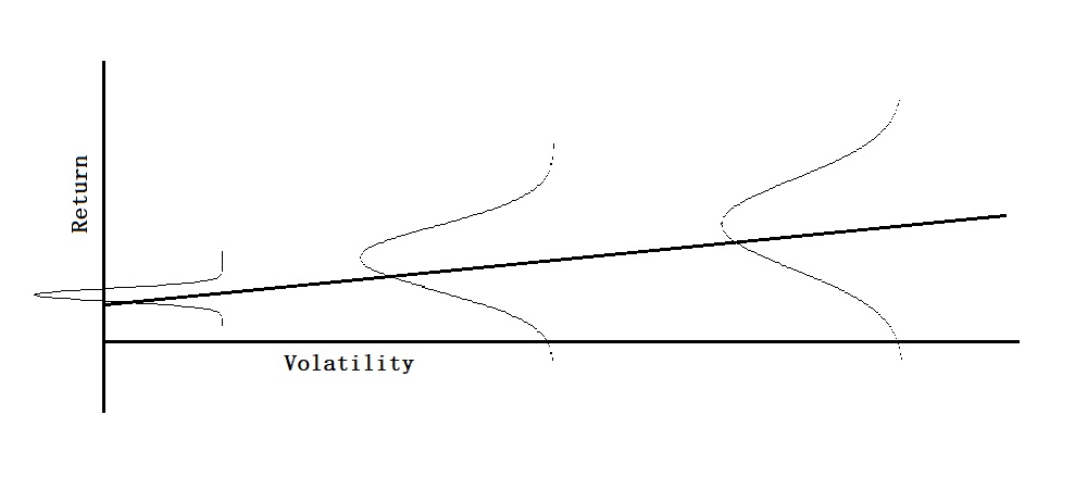
While the expected returns, the mean of the distribution, are higher to the right, the chances of higher and lower returns (including losses) are also higher. The critical issue here is that no one knows the breadth of the distribution or its shape. Imagine if it is what Nassim Taleb calls a fat tail, an asymmetric distribution, or the occurrence of a heavy impact-low probability event.

Reference

Howard Mark’s Memo on Risk

The Capital Market Line: Illusion of Return Read More »

Risk and Return – The Capital Market Line

We have seen how simple portfolio theory explains the relationship between risk and returns. For example, the representation below.

This leads to the development of what is known as the Capital Market Line (CML). CML is a concept that combines the risk-free asset and the market portfolio. It is the line connecting the risk-free return and tangent to the ‘efficient frontier’ of the portfolio.

The slope of the Capital Market Line (CML) is the Sharpe Ratio of the portfolio.
Sharpe Ratio = (Return of the portfolio – risk-free rate) / Standard deviation

But there is something wrong with this line – or at least how people perceive the line of risk vs return. That is, next.

Risk and Return – The Capital Market Line Read More »

Duel – Backward Induction

In the previous post, we developed the condition for the player to shoot the opponent. I.e., the distance (d*) at which the probability of the player who gets the turn is greater than or equal to the chance of the opposite missing in the next turn.

When the player, say P1, reaches d*, she can believe in two things. 1) P2 will not shoot in the next turn (d*-1) or
2) P2 will shoot in the next turn.
In the first case, P1 should not shoot. In the second case, P1 assesses that P1(d*) + P2(d*-1) = 1. So, P1 must shoot.

But what should Player 1 believe? The answer comes from backward induction.

Imagine the players came in close range (d = 0), and it’s P2’s turn. P2 will shoot and win. Taken one step back: P1 knows that in the next step, P2 will shoot, so she takes option 2. She assesses that P1(1) + P2(0) > 1, and she shoots. Go back one more step. Now, P2 knows that P1 will shoot in the next step, and if the distance is less than d*, P2 must shoot. It will continue until d* is reached.

Duel – Backward Induction Read More »

Duel

There are two players in the duel game, P1 and P2. Each carries a pistol loaded with a single bullet positioned a certain distance apart. Each player gets one round at a time, one after another. A player can shoot the other or step forward in her turn. Whoever hits the other wins the game. So, the player’s strategic decision is when she should shoot.

Let Pi(d) be the probability that player i will get her target (the opponent) from a distance d. The two players can have different abilities. In other words, P1(d) can be lower (or higher) than P2(d). Also, at d = 0, P1 and P2 hit the target (P1(0) = P2(0) = 1).

So, who will take the shot first, and when?

Imagine it’s P1’s turn, and she can believe in the following two things:
1) P2 will not shoot in the next turn
2) P2 will shoot in the next turn

If P1 believes in option 1 (that P2 will not shoot in the next turn), P1 will not shoot in this turn. If P1 thinks that P2 will shoot, then P1 will evaluate her options in the following manner. If P1 thinks her probability of hitting the target in this turn is greater than or equal to her opponent’s chance to miss in the next turn, she will shoot. Mathematically, that is:

P1(d) >/= 1 – P2(d-1) or
P1(d) + P2(d-1) >/= 1

The distance at which the condition is satisfied is d*. From the picture, it is clear that below d*, the probability, P1(d) + P2(d-1) > 1 and above d*, it is < 1.

Duel Read More »

Only Trade-Offs

American economist and political commentator Thomas Sowell summarises the core of decision-making, like nobody has, in his famous quote: There Are No Solutions, Only Trade-offs.

A crucial thing in trade-off is the assessment of the consequence of each option. A common practice in investment decisions is the cost-benefit analysis.

Only Trade-Offs Read More »

Logistic Regression and R

We have seen logistic regression as a means to estimate the probability of outcomes in classification problems where the response variable has two or more values. We use the ‘Default’ dataset from ‘ISLR2’ to illustrate. The data set contains 10000 observations on the following four variables:

default
: A factor with levels No and Yes indicating whether the customer defaulted on their debt

student:
 factor with levels No and Yes indicating whether the customer is a student

balance: 
The average balance that the customer has remaining on their credit card after making their monthly payment

income: Income of customer

We change YES to 1 and NO to 0 and plot default vs balance.

Let p(X) be the probability that Y = 1 given X. The simple form that fits this behaviour is:

P(X) = \frac{e^{\beta_0 + \beta_1 X}}{1 + e^{\beta_0 + \beta_1 X}}

The beta values (the intercept and slope) are obtained by the ‘generalised linear model’, glm function in R.

D_Data <- Default
D_Data$def <- ifelse(D_Data$default=="Yes",1,0)
model <- glm(def ~ balance, family = binomial(link = "logit"), data = D_Data)
summary(model)

Call:
glm(formula = def ~ balance, family = binomial(link = "logit"), 
    data = D_Data)

Deviance Residuals: 
    Min       1Q   Median       3Q      Max  
-2.2697  -0.1465  -0.0589  -0.0221   3.7589  

Coefficients:
              Estimate Std. Error z value Pr(>|z|)    
(Intercept) -1.065e+01  3.612e-01  -29.49   <2e-16 ***
balance      5.499e-03  2.204e-04   24.95   <2e-16 ***
---
Signif. codes:  0 ‘***’ 0.001 ‘**’ 0.01 ‘*’ 0.05 ‘.’ 0.1 ‘ ’ 1

(Dispersion parameter for binomial family taken to be 1)

    Null deviance: 2920.6  on 9999  degrees of freedom
Residual deviance: 1596.5  on 9998  degrees of freedom
AIC: 1600.5

Number of Fisher Scoring iterations: 8

Now, we will test how good the model predictions are by plotting the function using the regressed beta0 ( = -10.65) and beta1 (= 0.0055).

plot(D_Data$balance, D_Data$def, xlab = "Balance", ylab = "Default")

y <- function(x){
  exp(-10.65+0.0055*x) / (1 + exp(-10.65+0.0055*x))
}

x <- seq(0, 3000)
lines(x, y(x), col = "red")

But R has an even simpler way to get this curve.

plot(D_Data$balance, model$fitted.values)

Logistic Regression and R Read More »

Counting Humans Ever Existed

The world’s human population is so large that the number of people alive today exceeds the number of people who died in the past!” Surely, you must have heard such claims. But how many of you have verified the truth behind such statements? Well, the Population Reference Bureau (PRB) do have estimates on it.

The number of people who ever lived is related to three factors:

  1. The duration of human existence
  2. The average number of people at different periods in history
  3. The birth rate during each period.

The duration of human existence

The assumption was made based on the current evidence that modern Homo sapiens appeared around 190,000 B.C.E., originated in Africa.

The average number of people

Available information/estimations about the world populations in different eras of human history are collected.

YEARPOPULATION
190,000 B.C.E2
50,000 B.C.E.2,000,000
8000 B.C.E.5,000,000
1 C.E.300,000,000
1200450,000,000
1650500,000,000
19001,656,000,000
20006,149,000,000
20227,963,500,000

Birth rate (BR)

Humans’ average life expectancy (LE) has stayed at about 12 years for most of history. Twelve years translates to 1000/12 ~ 80 births per year per 1,000 population. The number has since improved to the present value of 17. This equation (BR = 1000/LE) works in a stable population.

Once the birthrates are available at the different periods, one can assume a stable population between intervals and estimate the births each year (in between those intervals) as
the number of years (between two periods) x BR x average population /1000

The estimated cumulative number of humans as of 2022 was 117,020,448,575. In other words, today’s world population of 7,963,500,000 (2022) is 6.8% of all homo sapiens ever lived.

Reference

How Many People Have Ever Lived on Earth?: prb.org

Counting Humans Ever Existed Read More »

Survival in a Truel

Anna, Bob and Claire are doing a three-way duel (a truel). Anna has an accuracy of 1/3, Bob has 2/3, and Claire is an excellent marksman with 1 (100%) accuracy. They must take turns shooting. Since each player knows others’ skills and all are rational, what would Anna do in the competition?

If Anna starts the duel and aims at Bob, there is a 1/3 chance she will shoot Bob. In that case, Claire has the next turn and will end Anna. On the other hand, if Anna aims at Claire, there is a 1/3 chance that Bob gets a chance to aim at Anna and end her with a 2/3 chance. So, it is clear that missing shots is a better option for Anna. So, she must shoot in the air first.

In the next chance, Bob will aim at the more prominent threat, i.e., Claire. Then there is a 2/3 chance of a showdown with Anna and a 1/3 chance that the showdown will be between Anna and Claire. Let P(A) be the probability that Anna survives, P(A, B) be the chance Alice wins the duel with Bob and P(A, C) Alice wins against Claire.

P(A) = 2/3 x P(A, B) + 1/3 x P(A, C)
P(A) = 2/3 x 3/7 + 1/3 x 1/3 = 25/63

Survival in a Truel Read More »

The sum of Dice – 5 before 7

The game is to roll a pair of dice until a sum of 5 or 7 is reached. Then, what is the probability that a sum of 5 comes before a sum of 7?

We use a few handly R commands to answer the problem.

1. expand.grid: gives all combinations of vectors – in our case, two dice.

rolls <- expand.grid(seq(1,6), seq(1,6))

2. do.call: executes a function on a list of arguments, e.g. to perform + (sum) to the earlier list.

sum_rolls <- do.call(`+`, rolls)
2  3  4  5  6  7  3  4  5  6  7  8  4  5  6  7  8  9  5  6  7  8  9 10  6  7  8  9 10 11  7  8  9 10 11 12

3. table function to tabulate each categorical variable (2 to 12) with its frequencies.  

tab_rolls <- table(sum_rolls)
sum_rolls
 2  3  4  5  6  7  8  9 10 11 12 
 1  2  3  4  5  6  5  4  3  2  1 

The table shows that the sum 5 occurs 4 times, and 7 can occur 6 times (out of the 36 possibilities). So, the probability of getting a five before seven (as the sum) is 4/(4+6) = 40%.

Combining steps into 2 lines.

dice_roll <- as.data.frame.table(prop.table(table(do.call(`+`, expand.grid(seq(1,6), seq(1,6))))))
dice_roll$Freq[which(dice_roll$Var1 == 5)] / (dice_roll$Freq[which(dice_roll$Var1 == 5)] + dice_roll$Freq[which(dice_roll$Var1 == 7)])

The sum of Dice – 5 before 7 Read More »

Another Dice Puzzle

A regular die has six sides, and the probability of getting a six is 1/6. If the die is modified so that the number 6 now appears to be half than usual (the frequency is halved), what is the probability of rolling a 6?

dice, roll the dice, to play-2031512.jpg

The question implies that the probability of getting 6 is half that of the other probabilities (1 to 5). Let p6 be the probability of rolling a six. Let p be the probability of rolling any other side.

For the die:
5 x p + p6 = 1
given p6 = p/2
5 x p + p/2 = 1
11p = 2
p = 2/11
p6 = p/2 = 1/11

The probability of rolling a six is not 1/12 but 1/11.

Another Dice Puzzle Read More »