Disease Spreading through Friendship

You saw friendship paradox as a concept, including its mathematics, but might be wondering if that had any real-life significance. Here is one interesting publication by Christakis and Fowler, who used this feature to predict pandemics.

The researchers monitored the friends of randomly selected individuals for the propagation of an outbreak. The hypothesis was that the illness spreads through the centrally located individuals, who have more connections than the peripheral ones. In such cases, the scientists expected, the S-shaped epidemic curve would shift to the left side (earlier times) for the more well-connected people, who are, as we know, the friends of friends in a friendship network.

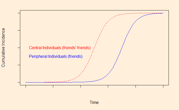
And that literally happened. The investigators monitored the propagation of H1N1 (and seasonal flu) from September 1 to December 31, 2009, at Harward college. Note that H1N1 had started in the US a few months earlier. A group of 744 undergraduate students participated in the study. The students were divided into two groups 1) randomly selected individuals (319) and 2) their friends (425) as named by the random group.

The results showed that the cumulative incident curve for the ‘friends’ group occurred 13.9 days earlier than that of the random group, paving the way for a potential means for the early detection (and intervention) of outbreaks.

Christakis, N. A.; Fowler, J. H., Social Network Sensors for Early Detection of Contagious Outbreaks

Disease Spreading through Friendship Read More »
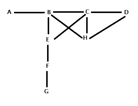
The Weighted Average paradox

If there is one statistical feature that links all three topics we have discussed in the last three days, starting with the inspection paradox, it will be the weighted average. In simple terms, if you make a random attempt to make a selection, your choice will be over-represented by the heavies. Be it a survey on classes, connecting to friends on social media or the waiting time for buses.

Think about a fortune wheel as depicted below. It’s spinning fast, and you come and touch the surface to stop it. Based on the number inscribed on the section, you get points. Note that the area of the cell is proportional to the number.

Without this information, you would have assumed the (expected) average prize to be 100/5 = 20. But when you look at the figure, you notice that the chances of hitting the different sections are not equal but related to the number on the wheel. To repeat the phrase that we have started with – it is proportionally over-represented by the heavies.

The expected value must take the probabilities. And thefore, it becomes 0.4 x 40 + 0.05 X 5 + 0.20 x 20 + 0.25 x 25 + 0.1 x 10 = 27.5

The Weighted Average paradox Read More »

Friendship Paradox

You know, your friends, on average, have more friends than you do! I know it is a bit difficult to swallow that feeling. We will explore it mathematically. On the one hand, it follows from what we have seen before – the inspection paradox and the waiting-time paradox. But we will use a different approach here.

Count your friends

Consider the following relationship tree.

What it means is that A has only one friend (i.e., B) denoted by A(1; B). Similarly B(4; A, C, E, H), C (4; B, D, E, H), D(2; C, H), E(3; B, C, F), F(2; E, G), G(1; F), H(3; B, C, D). So the total number of friends among those eight is 1 + 4 + 4 + 2 + 3 + 2 + 1 + 3 = 20. The average number of friends, therefore, is 20/8 = 2.5.

And their friends

How do we do it? The easier way is to call out each of them and ask how many friends they have. For example, take A: she will ask her only friend, B, to call out her friends. B has four friends (note that it also includes A). Let us represent that as A{B(4)}. Similarly, B{A(1), C(4), E(3), H(3)}, C {B(4), D(2), E(3), H(3)}, D{C(4), H(3)}, E{B(4), C(4), F(2)}, F{E(3), G(1)}, G{F(2)}, H{B(4), C(4), D(2)}. The total number is 60. To calculate the average friends’ friends, you should divide 60 by the friends you calculated earlier, i.e., 20. 60/20 = 3.

So by counting, you prove that the average number of friends (2.5) is smaller than friends’ friends (3). The whole exercise can be summarised in the following table

IndividualFriends
(P)
Friends’ friends
(Q)
Mean
Friends’ friends
(P/Q)
A1 44
B4 112.75
C4123
D273.5
E3103.33
F242
G1 22
H3103.33
Total206023.91

Analytical Proof

Look at the diagram once more. We replace the number of friends that A have with dA (dA represents the degree of the vertex that points from person A).

\\ \text{In other words, the total number of friends here is }, \\\\ d_A + d_B + d_C + d_D + d_E + d_F + d_G + d_H } =  \Sigma{x_i}

which we know is 20. The average number of friends is obtained by dividing this by the total number of individuals, n.

\\ \frac{d_A + d_B + d_C + d_D + d_E + d_F + d_G + d_H}{n} = \frac{\Sigma{x_i}}{n}

Now, we will move to the total friends of friends.

\\ \text{the number of friends that A's friends have = } d_B \\ \\  \text{the number of friends that B's friends have= } d_A + d_C + d_E + d_H \\ \\  \text{the number of friends that C's friends have= } d_B + d_D + d_E + d_H \\ \\  \text{the number of friends that D's friends have= } d_C + d_H \\ \\  \text{the number of friends that E's friends have= } d_B + d_C + d_F\\ \\  \text{the number of friends that F's friends have= } d_E + d_G \\ \\  \text{the number of friends that G's friends have= } d_F \\ \\  \text{the number of friends that H's friends have= } d_B + d_C + d_D \\ \\  \text{Total number of friends that all friends have= }   d_B+ d_A + d_C + d_E + d_H + d_B + d_D + d_E + d_H +  d_C + d_H + d_B + d_C +  d_E + d_G +  d_F + d_B + d_C + d_D = \\ \\ d_A + 4 d_B + 4 d_C + 2 d_D + 3 d_E + 2 d_F + d_G + 3 d_H \\ \\ \text{the average number of friends of friends is = } \frac{d_A + 4 d_B + 4 d_C + 2 d_D + 3 d_E + 2 d_F + d_G + 3 d_H}{d_A + d_B + d_C + d_D + d_E + d_F + d_G + d_H}

which was 60/20 in our case. If you are confused, remember these:

the total number of individuals = n
the avg. number of friends of individuals = total number of friends / total number of individuals
the avg. number of friends of friends = total number of friends of friends / total number of friends

Back to the equations.

\\ \text{the average number of friends of friends = } \\\\ \frac{d_A + 4 d_B + 4 d_C + 2 d_D + 3 d_E + 2 d_F + d_G + 3 d_H}{d_A + d_B + d_C + d_D + d_E + d_F + d_G + d_H}

Look carefully, dA appears once in the numerator, and dA has one friend (B). dB appears four times and dB has four friends, and so on. This is no accident as the number of friends is counted multiple times as they appear in the friends’ friends list. Apply this rule to the equation, and you get.

\\ \text{the average number of friends of friends = } \\\\ \frac{d_A*d_A + d_B*d_B + d_C*d_C + d_D*d_D + d_E*d_E + d_F*d_F + d_G*d_G + d_H*d_H}{d_A + d_B + d_C + d_D + d_E + d_F + d_G + d_H} \\ \\ = \frac{d_A^2 + d_B^2 + d_C^2 + d_D^2 + d_E^2 + d_F^2 + d_G^2 + d_H^2}{d_A + d_B + d_C + d_D + d_E + d_F + d_G + d_H} \\ \\ = \frac{\Sigma{x_i^2}}{\Sigma{x_i}} \\ \\ \text{divide the numerator and the denominator by n} \\ \\  =  \frac{\Sigma{x_i^2}/n}{\Sigma{x_i}/n} \\ \\ \text{add and subtract } (\Sigma{x_i})^2/n^2 \text { at the numerator} \\ \\  =  \frac{[\Sigma{x_i^2}/n +  (\Sigma{x_i})^2/n^2  -   (\Sigma{x_i})^2/n^2]}{\Sigma{x_i}/n} \\ \\ =  \frac{[\Sigma{x_i^2}/n  -   (\Sigma{x_i})^2/n^2]}{\Sigma{x_i}/n} +  \frac{[(\Sigma{x_i})/n]^2}{\Sigma{x_i}/n} \\ \\ =  \frac{[\Sigma{x_i^2}/n  -   (\Sigma{x_i})^2/n^2]}{\Sigma{x_i}/n} + {\Sigma{x_i}/n}

The second term, we know from the earlier section, is the average number of friends of individuals. The first term is nothing but the variance divided by the mean.

The mean number of friends of friends = (mean of friends ) + (variance / mean), which is equal to or greater than the mean of friends.

References

Why do your friends have more friends than you do? The American Journal of Sociology

The friendship paradox: MIT Blossoms

Friendship Paradox Read More »

Waiting-Time Paradox

Have you ever wondered why you always had to wait longer at the bus stop? If you agree with that but feel it was more of a mental thing than anything else, hold on a bit. There are chances that your feeling is valid and may be explained using probability theory.

Remember the inspection paradox?

See the previous post if you don’t know what I am talking about. The waiting time paradox is a variation of the inspection paradox. And we will see how, so brush up on your probability and expected value basics. As a one-line summary, the expected value is the average value!

A bus every 10 minutes

You know a bus for your destination comes every 10 minutes at a bus stop. In other words, six buses every hour. You start with the premise that the average waiting time is five minutes, assuming you randomly reach the stop. One day, at one minute for the next bus (waiting time 1 min) or another day, a minute after the last bus (waiting time = 9 min), etc.

Do not forget that buses also come with certain uncertainties (unless your pick-up is at the starting station). Now, let’s get the arrival times of this bus at a given stop (at some distance after the starting point). I can make them up for illustration but will, instead, resort to the Poisson function and get random time intervals between two consecutive buses.

Here they are: made using the R code, “rpois(6, 10)“: 10, 10, 11, 3, 10, 16. These are minutes, inside an hour, between buses, created randomly. The code [rpose(N = sample Size, lambda = expected interval)] randomly generated 6 intervals at a mean value 10.

The average waiting times inside these six slots are 10/2, 10/2, 11/2, 3/2, 10/2 and 16/2. You know what happens next.

Probabilities and expectations

Compute your probability of catching a bus during that hour. They are 10/60, 10/60, 11/60, 3/60, 10/60 and 16/60. Each number on the numerator corresponds to a slot and a time between two buses, which equals the respective waiting time, as described in the previous paragraph.

The expected value (average waiting time) = Probability x average waiting time corresponding to that probability = (10/60) x (10/2) + (10/60) x (10/2) + (11/60) x (11/2) + (3/60) x (3/2) + 10/60 x (10/2) + (16/60) x (16/2) = 5.72.

Average is > 5 minutes

The following code summarises the whole exercise.

number_of_buses <- 100 
avg_wait_buses <- 10

bus_arrive <- rpois(number_of_buses, avg_wait_buses )
prob_bus_slot <- bus_arrive/sum(bus_arrive)
avg_wait_slot <-  bus_arrive / 2
Expected_wait <- sum(prob_bus_slot*avg_wait_slot)

Waiting-Time Paradox Read More »

Inspection Paradox

Suppose a school has three classes, A, B and C, holding 20, 60 and 100 students. What is the average number of students in a class? Well, it depends on who you ask. Let’s understand this deeper.

If you ask the school principal, she will give you 60 as the average number. It’s simple, (20 + 60 + 100) / 3 = 60. But what happens if you choose to sample 50 students and ask them about the number of students in their classes and then average it?

You wait at the school bus stop and randomly select 50 students. Since the sampling is random, you are likely to catch the following numbers from each class.

The probability of finding a student from class A = (20/180). Therefore, the number of students from class A in the total sample of 50 = 50 x (20/180) = 5.55, about 6.

Similarly, from class B, you catch 50 x (60 / 180) = 16.66 or about 17 students, and from class C, 50 x (100 / 180) = 27.77 or about 28 students.

So what are the responses from the students? 5.55 will say 20 students in their class because they are from class A. 16.66 will say 60, and 27.77 says 100. So, the survey average is (5.55 x 20 + 16.66 x 60 + 27.77 x 100) / (5.55 + 16.66 + 27.77) = 3887.6 / 50 = 77.8.

So from the school, you get 60, and from the survey, 78, and no one is lying.

Inspection Paradox Read More »

Wisdom of the Crowd

Wisdom of the crowd is an intriguing phenomenon, which received its popularity in public discourse due to Galton when he surprisingly found a near-accurate estimate of the weight of a prize-winning ox by the common public. In other words, whatever errors in the guesses of the individuals got cancelled when averaged. An essential prerequisite of achieving the group’s wisdom is that the errors of individuals are statistically independent of each other.

Vul and Pashler took this to the next level. They wanted to test it for single individuals by allowing them to make multiple guesses. They asked 428 participants (through an internet poll) eight questions regarding general knowledge. Half of the participants were asked to make a second guess immediately after the questionnaire, and the other half were asked after three weeks (without telling them it would come after three weeks).

The results were surprising. The within-person average of the guesses (or the mean square error) was lower than either of the guesses for the immediate responders. The value was even lower for late-responders.

Wisdom of the Crowd Read More »

One-Son Policy

You may have heard about the one-child policy. Imagine if a country decides to have a one-son policy. The question is: will it lead to a gender imbalanced society? Intuition suggests that there will be more girls in the land because of this policy. Let’s analyse this by estimating the expected values.

The analytical solution

Assume that the probability of either sex is equal, 1/2. We have seen earlier that if p is the probability of something, then the expected value (denoted by E) or the average time we need to wait for the first success is 1/p. In our case, if N is the number of children in a family with 1/2 as the parameter, E(N) = 1/(1/2) = 2. Let Nm be the number of male children and Nf be the number of females, N = Nm + Nf and E(N) = E(Nm) + E(Nf) = 2. E(Nm) for a one-son policy regime has to be 1. That means E(Nf) = 2 – 1 = 1. So the expected number of males and females are equal! Not convinced? We will illustrate with examples.

Testing the concept

1 child scenario: The simplest case is one child in a family. The child can be M (male) or F (female). p(M) = 1/2, p(F) = 1/2. Nm(M) = 1, Nm(F) = 0, Nf(M) = 0, and Nf(F) = 1.

E(Nm) = Nm(M) x p(M) + Nm(F) x p(F) = 1 x (1/2) + 0 x (1/2) = 1/2.
E(Nf) = Nf(M) x p(M) + Nf(F) x p(F) = 0 x (1/2) + 1 x (1/2) = 1/2.
So the expected values of males and females are equal

A bit of explanation on the notation:
Nm(M) is the number of boys in an M scenario, and Nm(F) is the number of boys in an F scenario.
Nf(M) is the number of girls in an M scenario, and Nf(F) is the number of girls in an F scenario.

Maximum 2 children in a family: The combinations are M, FM, FF.
p(M) = 1/2, p(FM) = 1/4, p(FF) = 1/4
Nm(M) = 1, Nm(FM) = 1, Nm(FF) = 0
Nf(M) = 0, Nf(FM) = 1, Nf(FF) = 2

E(Nm) = Nm(M) x p(M) + Nm(FM) x p(FM) + Nm(FF) x p(FF) = 1 x (1/2) + 1 x (1/4) + 0 x (1/4) = 3/4.
E(Nf) = Nf(M) x p(M) + Nf(FM) x p(FM) + Nf(FF) x p(FF) = 0 x (1/2) + 1 x (1/4) + 2 x (1/4) = 3/4.
Again, the expected values of males and females are equal

Maximum 3 children in a family: The combinations are M, FM, FFM, FFF.
p(M) = 1/2, p(FM) = 1/4, p(FFM) = 1/8, p(FFF) = 1/8
Nm(M) = 1, Nm(FM) = 1, Nm(FFM) = 1, Nm(FFF) = 0
Nf(M) = 0, Nf(FM) = 1, Nf(FFM) = 2, Nf(FFF) = 3

E(Nm) = Nm(M) x p(M) + Nm(FM) x p(FM) + Nm(FFM) x p(FFM) + Nm(FFF) x p(FFF)
= 1 x (1/2) + 1 x (1/4) + 1 x (1/8) + 0 x (1/8) = 7/8.
E(Nf) = Nf(M) x p(M) + Nf(FM) x p(FM) + Nf(FFM) x p(FFM) + Nf(FFF) x p(FFF)
= 0 x (1/2) + 1 x (1/4) + 2 x (1/8) + 3 x (1/8)= 7/8.
Once again!

More Proof?

We will do one final time, where the family waits for a boy but stops at 4. The combinations are M, FM, FFM, FFFM, and FFFF.
p(M) = 1/2, p(FM) = 1/4, p(FFM) = 1/8, p(FFFM) = 1/16, p(FFFF) = 1/16.
Nm(M) = 1, Nm(FM) = 1, Nm(FFM) = 1, Nm(FFFM) = 1, Nm(FFFF) = 0
Nf(M) = 0, Nf(FM) = 1, Nf(FFM) = 2, Nf(FFFM) = 3, Nf(FFFF) = 4

E(Nm) = Nm(M) x p(M) + Nm(FM) x p(FM) + Nm(FFM) x p(FFM) + Nm(FFFM) x p(FFFM) + Nm(FFFF) x p(FFFF)
= 1 x (1/2) + 1 x (1/4) + 1 x (1/8) + 1 x (1/16) + 0 x (1/16) = 15/16.
E(Nf) = Nf(M) x p(M) + Nf(FM) x p(FM) + Nf(FFM) x p(FFM) + Nf(FFFM) x p(FFFM) + Nf(FFFF) x p(FFFF)
= 0 x (1/2) + 1 x (1/4) + 2 x (1/8) + 3 x (1/16) + 4 x (1/16) = 15/16.
Still, there is a balance between boys and girls

One-Son Policy Read More »

Hot Hands of Randomness

A lot of basketball fans believe in hot hands and streak shooting. These phrases roughly suggest the probability of a basket is higher following a hit than a miss. A spectator suddenly gets confidence in a player who shot the previous two shots to make the next. At that moment, she would not think about probabilities (coin tossing games) but only consider the momentum and confidence of the shooter.

It is interesting to notice that this behaviour of the fans is just the opposite of the belief in “the law of small numbers” or the gambler’s fallacy. The reason: basketball is being played by individuals with flesh and blood (and lucky charm), whereas gambling is by machines that work on chances (and expected values).

In 1985, Gilovich et al. did a study that analysed the data from 48 home games of the Philadelphia 76ers and their opponents during the 1980-81 season. The following is what they found.

The first table is about the (conditional) probability of a hit, given the player had already hits (3, 2 and 1). P(hit) represents the overall shooting percentage of the player.

P(hit)P(hit|3H)P(hit|2H)P(hit|1H)
Richardson0.500.480.500.49
Erving0.520.480.520.53
Hollins0.460.320.460.46
Cheeks0.560.590.540.55
Jones0.470.270.430.45
Toney0.460.340.400.43
Jones0.540.530.470.53
Mix0.520.360.480.51
Dawkins 0.620.510.580.57

Similar statistics for a player to hit after missing the previous shots are presented below.

P(hit)P(hit|3M)P(hit|2M)P(hit|1M)
Richardson0.500.500.470.56
Erving0.520.520.510.51
Hollins0.460.500.490.46
Cheeks0.560.770.600.60
Jones0.470.500.480.47
Toney0.460.520.530.51
Jones0.540.610.580.58
Mix0.520.700.560.52
Dawkins 0.620.880.730.71

The data showed just the opposite of what people believed. The hits following previous hits were lower than previous misses.

Gilovich, T.; Vallone, R.; Tversky. A., Cognitive Psychology 17, 295-314 (1985)

Hot Hands of Randomness Read More »

Whose Fault was It?

A company gets their tools from three factories, 10% from F1, 50% from F2 and 40% from F3. The fault rates of the three factories are 2.5%, 1.5% and 1%, respectively. If the company finds one of the tools defective, from which factory is it likely?

Let’s write down things in the proper format and test the probabilities, one by one. Let P(F1|D) be the probability that the tool came from F1 given the information (that it is faulty), P(D|F1), the fault rate of F1 and P(F1) is the prior chance of F1 in the company.

\\ P(F1|D) = \frac{P(D|F1)*P(F1)}{P(D|F1)*P(F1) + P(D|F2)*P(F2) + P(D|F3)*P(F3)}  \\ \\ P(F2|D) = \frac{P(D|F2)*P(F2)}{P(D|F1)*P(F1) + P(D|F2)*P(F2) + P(D|F3)*P(F3)}  \\ \\ P(F3|D) = \frac{P(D|F3)*P(F3)}{P(D|F1)*P(F1) + P(D|F2)*P(F2) + P(D|F3)*P(F3)}

I guess you already know that I applied Bayes’ theorem to each factory. Now, add numbers and solve.

\\ P(F1|D) = \frac{0.025*0.1}{0.025*0.1 + 0.015*0.5 + 0.01*0.4}  = \frac{0.0025}{0.014} = 0.18\\ \\ P(F2|D) = \frac{0.015*0.5}{0.025*0.1 + 0.015*0.5 + 0.01*0.4}  = \frac{0.0075}{0.014} = 0.54\\ \\ P(F3|D) = \frac{0.01*0.4}{0.025*0.1 + 0.015*0.5 + 0.01*0.4}  = \frac{0.004}{0.014} = 0.29

The tool is more likely to have come from F2.

Whose Fault was It? Read More »

Coin Tossing and NBA Playoffs

In the previous post, we have established the expected probabilities of the winning margins in the NBA playoffs. This time we compare them with the past data and test our hypothesis.

The null hypothesis (H0) was that the games-outcomes occur with equal probabilities, irrespective of the rank in the regular season. The alternative hypothesis (H1) says that the game outcomes are not at equal chances but based on the team’s strength.

Matches including round 1

We gather all the playoff outcomes until 2021, from the starting point of 2003, the beginning year of the best-of-seven series for round one. The summary of the observed results and expectations is in the following table.

Observed (O)Expected (E)(O-E)2/E
4-game series520.125 x 285
= 35.63
7.52
5-game series740.25 x 285
= 71.25
0.106
6-game series990.3125 x 285
= 89.06
1.109
7-game series600.3125 x 285
= 89.06
9.48
Total28528518.21
obsfreq <- c(52,74, 99, 60)
nullprobs <- c(0.125,0.25, 0.313, 0.312)
chisq.test(obsfreq,p=nullprobs)

Not among equals

With a chi2 of 18.2 (> the critical value of 7.81 for the 5% significance level) and a p-value of 0.00042, we reject the null hypothesis that the playoff games were coin-tosses. The results are hardly surprising because of the presence of first-round playoffs in the data. Most of the matches in the first round are not played among equals. In the first round, the number one (of the regular season) plays against the number 8, 2 against 7, 3 against 6, and 4 against 5. With a closer review of the table, you can see far more 4-0 results (52) than expected (35) and fewer 4-3s (60) than coin-tosses (89).

After the first round

Once the screener of the first round is completed, it is the start of the conference semi-finals. We now anticipate that the matches are between equals or teams of comparable strength. We repeat the test by taking data from 2003 to 2021, excluding the first round. The analysis is below.

Observed (O)Expected (E)(O-E)2/E
4-game series190.125 x 132
= 16.5
0.38
5-game series300.25 x 132
= 33
0.27
6-game series520.3125 x 132
= 41.316
2.76
7-game series310.3125 x 132
= 41.316
2.52
Total1321325.93

The chi2 is below the critical value (7.81), corresponding to a 5% significance level. Yes, the null hypothesis stays.

The final

We will now take it to the next level. Let’s cover only the NBA finals of the last 75 years. We expect the outcome to match that of matching probability events. And the expected chi2 value could be the lowest we have seen so far. Keep your fingers crossed.

Observed (O)Expected (E)(O-E)2/E
4-game series90.125 x 75
= 9.37
0.015
5-game series180.25 x 75
= 18.75
0.03
6-game series290.3125 x 75
= 23.44
1.3
7-game series190.3125 x 75
= 23.44
0.83
Total75752.17

Yes, it is – chi2 of 2.17 with a p-value of 0.54.

Coin Tossing and NBA Playoffs Read More »