We have seen the birthday problem more than once. It was initially a difficult proposition to accept that it takes only 40 people to have a match of birthdays (with 90% probability). That comes from a misconception about randomness. You have assumed that randomness meant things must spread out equally. In other words, there should be close to 365 people for two people sharing a birthday. In random processes, clustering is so natural, whereas non-clustering requires effort.
Think about an experiment in which 365 boxes lie in a line. And balls are falling from the sky. What is the probability that these balls will fill equally in each box? It is so hard for the falling balls to distribute equally without aggregation. And the reason? It’s random, and there is no brain behind the fall!
We have already seen decision making based on expected value and utility functions (of gains and losses). The typical stories consider isolated affairs, but real life is full of connected events. The real question is how and whether prior losses and gains influence the behaviour of the decision-maker.
In gambling, it has been found that prior gains can increase willingness to gamble more (house money effect), and previous losses do the opposite. It is on that premise that Thaler and Johnson conducted experiments and asked the participants the following questions.
Mr A was given two lotteries. He won $50 in one and $25 in another. Mr B was given one lottery and won $75. Who was happier? 64% of the subjects thought A was happier.
Mr A received a letter from the tax authorities that he made a mistake in the returns and was required to pay $100. He received another note on the same day for another $50. Mr B got one letter from the authorities for $150. Who was more upset? 75% of the participants thought it was A.
Mr A’s car was damaged in a parking lot and had to spend $200 on repairs. The same day he won a lottery for $25. Mr B’s car was damaged and he had to spend $175. Who was more upset? 70% answered B.
Mr A won a lottery for $100, but on the same day, he damaged the rug in his apartment and had to pay $80 to his landlord. Mr B bought a lottery and won $20. Who was happier? An overwhelming majority thought it was B.
Richard Thaler and Eric Johnson, “Gambling with the House Money and Trying to Break Even: The Effects of Prior Outcomes on Risky Choice”, Management Science, 1990.
Do you have a problem supporting the political, economic, and social equality of women? Well, I don’t, and if I were to believe what countless surveys all over the world suggest, most of us, too, don’t have any problem.
But what if I say that the above statement is the textbook definition of feminism? Now, assuming you represent various poll results on this topic, you may have changed your view – from the position of approval to that of disapproval. The term has a poor approval rate all over the world. Feminism is a case where the definition, the way we all perceive it, is defined by its opponents!
Why is it not cool?
Let’s understand what went wrong with such a dignified concept. Feminism is a story of so many biases and fallacies. It has straw man (woman) fallacy, cherry-picking, fear of the unknown, stereotyping; you name it.
Straw woman fallacy
Popular culture – movies and TV – do their part to misrepresent the position to make it easier to critique. They can easily morph feminists into a myriad of effigies such as socialists (in the US), lesbians, child-killers, and man-haters that are thus easier to attack and burn down.
Take the case of the bra-burners. It was down to a journalist who erroneously reported the incident of burning of bras in a protest in 1968, when a few women threw some brassieres into the thrash can in protest of the Miss America pageant.
Fear of unknown
Yes, feminism does threaten the existing power centres. Be it the patriarchy, sexuality, or individual rights. More importantly, this fear of losing the value system or privilege that society thinks they enjoy currently, is what most of us are worried about. Like nationalism, like the belief in God, this concept of, often male-created, value system too, remains in the head, as a myth, without undergoing any rational scrutiny.
The fallacy of selective attention
There are feminists, past and present, who walked the elitist and exclusionist paths. But whenever such extreme expressions happened, the press made sure that they got more publicity than they deserved.
There are two approaches to statistical inference, and we have briefly touched upon those in the past. They are the frequentist approach and the Bayesian approach.
Frequentists count the occurrences and estimate probability as the limiting frequency. They take random samples from the population and find fixed parameters (theta) of the distribution. Their objective is to create the confidence interval and capture the parameter inside it.
If you repeat the experiment several times, you trap theta 95% of the time.
For Bayesians, on the hand, the probability is often a subjective belief. And parameters are random variables. They take the entire data intending to get the updated chance of the parameters.
However, you will not trap the parameter 95% of the time if you repeat the experiment.
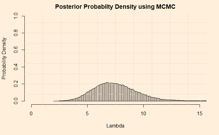
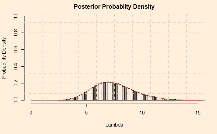
In the last post, we developed an MCMC algorithm for calculating the posterior probability distribution for the shark problem. We will do a few more things on it before closing out.
The first thing is to express the histogram in the form of Gamma distribution. We calculate the mean and variance of the data and apply the following formulae.
Now, check the post where we did the analytical solution for the hyperparameters of the posterior. Do they match?
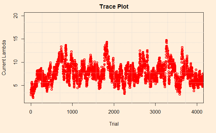
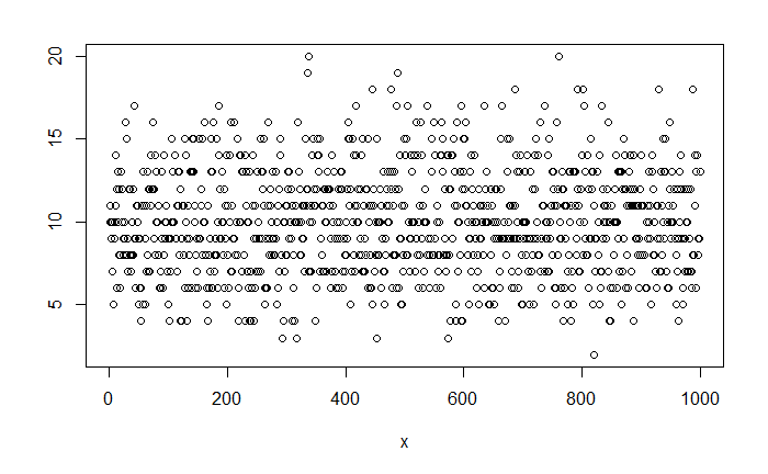
Trace Plot
Trace plot is next. It is a line diagram connecting all the current lambdas against the trial number. The following plot gives the first 4000 (of the 100,000) trials we have performed.
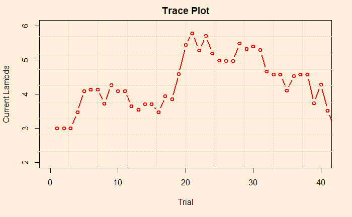
Now we pick the first 40 to zoom in on the values.
By looking at the plot, you may recognise the concept known as the acceptance rate. It is the percentage of instances where the current lambda got rejected in favour of the proposed. In the figure, there are approximately three in four times the points jumped (up or down) to a new value. There are recommendations to keep the acceptance rates between 25 – 50% as a good practice. You can tune the rate by varying the standard deviation of the normal distribution (step 3 of the MCMC scheme).
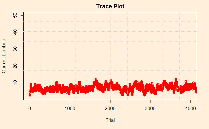
Impact of starting lambda
Finally, we look into the sensitivity of prior. We had arbitrarily chosen 3 in the previous exercise. Here is the trace plot once again.
What about changing it to 30? We could see that the distribution remained the same (after 100,000 iterations). Let’s check the trace plot. You will notice that it was higher, to begin with, but came down in a few trials.
Reference
Bayesian Statistics for Beginners: a step-by-step approach, Donovan and Mickey
So far, we have created an analytical solution to the Poisson-Gamma conjugate problem. Now, it is time for the next step: a numerical solution using the Markov Chain Monte Carlo (MCMC) method. The plan is to go stepwise and develop R codes side by side.
Markov Chain Monte Carlo
We write the Bayes’ theorem in the following form,
Step 0: The Objective
The objective of the exercise is to calculate the probability density of the posterior (updated hypothesis) given the (new) data at hand. As we did previously, we will need to use the hyperparameters alpha and beta.
data_new <- 10
alpha <- 5
beta <- 1
Step 1: Guess a Lambda
You start with one value for the posterior distribution (of lambda). It can be anything reasonable; I just took 3. It is an arbitrary selection. We can think of changing to something else later.
current_lambda <- 3
Step 2: Calculate the Likelihood, prior and posterior
Use the guess value of lambda and calculate the likelihood using Poisson PMF. In other words, get the chance of occurrence of a rare independent event 5 times in a year if the lambda was 3.
liklely_current <- dpois(data_new,current_lambda)
Calculate the prior probability density associated with the lambda (value of the posterior) for the given hyperparameters, alpha and beta. Sorry, I forgot: use Gamma PDF.
The next one is obvious, use the calculated values of prior and likelihood and calculate the probability density of the posterior using the new form of the Bayes’ equation.
post_current <- liklely_cur*prior_current
Step 3: Draw a Random Lambda
The second value of lambda is selected at random from a symmetrical distribution that is centred at the current value of lambda. We will use a normal distribution for that. We’ll call the new value, the proposed lambda. I used the absolute value because the new value can pick negative once in a while and lead the program to terminate.
Now you have two posterior values, post_current and post_proposed. We go to throw one out. How do we make that decision? Here comes the famous Metropolis algorithm to the rescue. It specifies to pick the smaller of the two between 1 and the ratio of the two posteriors. The resulting value is the probability of moving to the new lambda.
prob_move <- min(post_proposed/post_current, 1)
Step 6: New Lambda or the Old
The verdict (to move or not) is not out yet! Now, draw a random number from a uniform distribution and compare it. If your number is higher than the random number, move to the new lambda, and if not, stay with the old lambda.
You have done one iteration, and you have a lambda (switch to new or retain the old). Now, you go back to step 2 and repeat all steps. Thousands of times until you meet the set iteration number, for example, one hundred thousand!
n_iter <- 100000
for (x in 1:n_iter) {
}
Step 8: Collect All the Accepted Values
Ask the question: what is the probability density distribution of the posterior? It is the normalised frequency of lambda values. Note that I just omitted the condition, “given the data”, to keep it simple, but don’t forget, it is always the conditional probability. You may get the histogram from the frequency data using the attribute “freq = FALSE”. See below
We have created the background on the Shark attack problem to explain how Bayesian inference operates for updating knowledge of an event, in this case, a rare one. Let’s have a quick recap first. We chose Poisson distribution to describe the likelihood (the chances of that data on attacks, given a particular set of occurrences) because we knew these were rare and uncorrelated events. And the Gamma for describing the prior probability of occurrences as it can give a continuous set of instances ranging from zero to infinity.
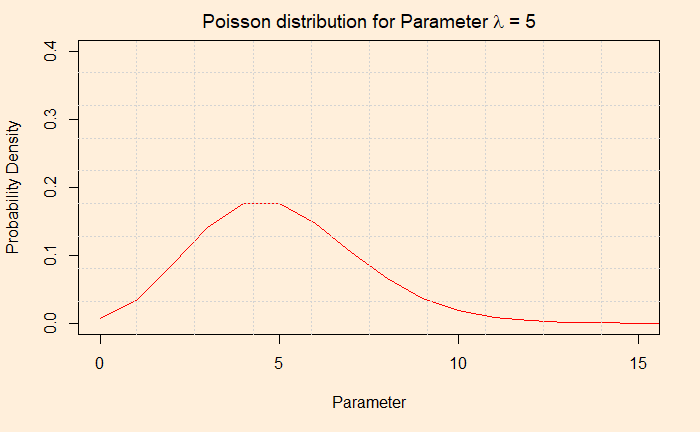
And if you like to know how those two functions work, see the following two plots.
The first plot gives the probability of one occurrence, two occurrences, 3, 4, 5, 6 …, when the mean occurrence is five. The value the X-axis take is discrete: you can not have the probability of 1.8 episodes of a shark attack!
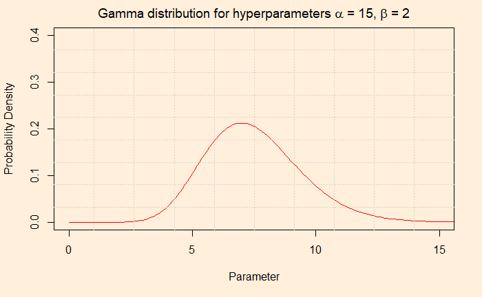
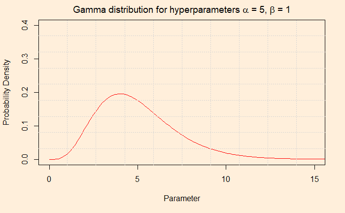
The second plot provides the probability of the parameter (occurrence or episode) through the gamma pdf using those two hyperparameters, alpha and beta.
Bayesian Inference
The form of Bayes’ theorem now becomes.
Then the magic happens, and the complicated looking equation solves into a Gamma distribution function. You will now realise the choice of Gamma as the prior was not an accident, but it was because of its conjugacy with the Poisson. But we have seen that before.
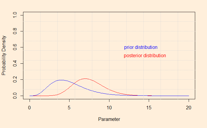
The Posterior
The posterior is a Gamma pdf with the following hyperparameters.
And, if you want to see the shift of the hypothesis from prior to posterior after the evidence,
This post will run in three parts. Here, we take a Bayesian inference challenge and analyse it analytically and numerically. I have followed the book “Bayesian Statistics for Beginners” by Donovan and Mickey for reference.
Bayesian Inference
The objective of Bayesian inference is to update the probability of a hypothesis by incorporating new data. The generic form of the Bayes’ theorem is written as:
The left-hand side of the equation represents the posterior distribution of a single parameter, theta, given the observed data. The first term on the numerator is called the likelihood, and the second term is the prior distribution (the existing knowledge before the arrival of the new data) of the parameter. We will soon see what I meant by parameter and how the (distribution) functions for the likelihood and prior are selected. Remember, the integral in the denominator is a constant; we will use that information soon.
Sharks and Poisson
Now the problem you want to solve: it is known that, on an average year, five shark attacks happen in a particular place. Last year it rose to ten. Do you think it is abnormal, and how do you update your database based on this data?
Shak attacks are rare. And they follow no pattern; in other words, one episode is independent of the previous one. Yes, you are guessing it right; I want to use the Poisson distribution to describe the likelihood of shark attacks. Although the word “poisson” means fish in French, the distribution got its name after the famous French mathematician Simeon Poisson!
The Parameter
In our case, based on the historical data, five attacks occur a year. Now, can the average five justify seeing ten last year? You either use the formula as seen in an earlier post or the R code, dpoise(10, 5). The answer is ca. 0.018. What about using a parameter value of 6 or 8? If you plug in those numbers, you will find they also lead to non zero probabilities. In other words, it is better to use a set of numbers (also called a distribution) instead of a single number as your prior. A gamma distribution can provide that set for two reasons, 1) it can give a continuous range of parameter values you wanted 2) the function is well suited with Poisson for solving the integral of the Bayes’ equation analytically. If you want to know what I meant, check this out.
The Gamma distribution function has two hyperparameters, alpha and beta. We use the word hyperparameters to distinguish from the other (theta), which is the unknown parameter of interest. Alpha/beta gives the mean. In our case, we settle for alpha = 5 and beta = 1 for the prior. The average (5/1 = 5) is matching with the existing data. You may as well consider 10 and 2, which also gives a mean of 5, but we stick to 5 and 1. Before we go and do the analysis, which is in the next post, check the parameter values that we will input to the Poisson to use.
People unaware of their own biases pose a clear threat to quality decision making. And we have discussed biases several times in the past. However, biases are also a result of our need to minimise energy spent on the thinking process. We will see what this means.
Scientists have hypothesised an explanation for this phenomenon along the lines of cognitive operations of the human system. They classify two types of thinking processes. They are 1) System one or intuitive thinking and 2) System two or reflective thinking.
In the first case, our actions flow effortlessly. Such as eating a piece of cake! Since we have evolved this way, it is not a complete surprise that energy-saving conserving modes of thinking got the default status (the brain consumes 20% of the body’s energy).
Reflective thinking, on the other hand, requires more energy. These are deliberate and slow, and you do it when the stakes are high. The primary focus is to reduce error, and therefore you are willing to spend your valuable energy. Remember our past as hungry hunter-gatherers.
To give an example, when someone learns how to ride a bike, “a very risky affair”, she is in system-two mode. A year later, as a master biker now, riding is her second nature, and it is now a system one process.
We have come across Poisson distribution a few times already. It is a way of estimating the probabilities of rare and independent events. But do you know Poisson is related to binomial distribution under certain circumstances?
But that should not come as a surprise. The binomial function estimates the probability of the number of successes in n discrete and independent trials, each with a chance of success = p. Whereas, Poisson gives the same but for rare events (events with low probabilities). In other words, Poisson is a special case of binomial when p is small ( p -> 0) and n is high (n -> infinity) (and its parameter lambda = n x p stays fixed). Let’s test this with an example.
A typist makes one mistake in every 500 words. If one page contains 300 words, what is the probability that she made no more than two mistakes in five pages?
Binomial
Start with Binomial for s occurrences in n trials.
P(X = s) in the equation should be read as: “what is the probability that a random variable called X has a value s”.
Poisson
Since p = 1/500 is small, and n = 1500 is high, we can apply Poisson. The mean of a binomial random variable is np, and we will substitute that as the parameter, lambda, representing the mean number of occurrences in a fixed period.
There is about a 42% chance that the error in five pages to remain not more than two.
Before we end, we should know the shortcuts to obtain the above results from the cumulative density functions (CDF). You may either look up the table or follow the R code.
![\\ C = \left[ \bar{X_n} - \frac{1.96}{\sqrt{n}}, \bar{X_n} + \frac{1.96}{\sqrt{n}} \right] \\ \\ \mathbb{P}_{\theta} (\theta \in C) = 0.95 \text{ for all } \theta \in R](https://thoughtfulexaminations.com/wp-content/ql-cache/quicklatex.com-5d2675e43009e980ef62c5dfcf06fe02_l3.png "Rendered by QuickLaTeX.com")