The 17 Coins Game

Another game Played between two players. In this case, 17 coins are placed in a circle. A player can take one or two coins in her turn. In the case of the two, they must be next to each other, i.e., there must be no gap between them. Whoever takes the last coin wins. Like before, the game offers an advantage to one person. Who is it, and what is her winning strategy?

Well, the advantage is with the second person. Here is the strategy: 

Case 1: the first person takes one coin

The second person must take two coins from the opposite side, breaking down the arc into two – with seven coins each. 
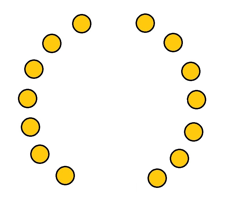
From now on, the game is simple: copy what the first person does on one of the arcs to the opposite arc. Since your turn is second, you will be the one who ends the game. 

Case 2: the first person takes two coins

The second person must also create two arcs with seven coins each by removing one from the diametrically opposite end. The rest is the same as before.  

Can You Take the Final Coin? A Game Theory Puzzle: William Spaniel

The 17 Coins Game Read More »

The 21 Flags Game

Here is a game played between two parties, each taking turns. There are 21 flags. The first person, in her turn, must pick up one, two or three flags—the game shifts to the second one to do the same. The game continues. The person who picks up the last flag is the winner. In theory, the game offers an advantage to one person. Who is it, and what is her winning strategy?

As with many games, this can also be solved by thinking backwards. Imagine only one flag remaining; the person whose turn comes up wins. The same is true for two and three flags, as she can take one, two, or three in her turn. Let’s denote that person – the first in line – 1.

1 wins 1, 2, 3

There are now four flags. Person 1 can remove one, two, or three, but the last chance is for person 2. 

1 lose: 4

If there are five flags, 1 can choose one flag, and 2 is left with a four-flag situation, i.e. 2 loses. The same is true for six and seven.

1 wins 1, 2, 3, 5, 6, 7

In the case of Eight Flags, if 1 takes one, two or three, 2 gets one of the winning numbers (8-1 = 7, 8-2 = 6 or 8-3 = 5).

1 lose: 4, 8

Continuing this pattern, person 1 can win when the flags in her turn are 1, 2, 3, 5, 6, 7, 9, 10, 11, 13, 14, 15, 17, 18, 19, and 21 and will lose when the flags are 4, 8, 12, 16, 20.

Since 21 is on person 1’s list, she can win this game by always picking the flags, leaving a multiple of four to the opponent. So, at the beginning of the game, the starter picks up one flag, leaving the opponent to choose next. Person 2 can leave 19, 18, or 17 for person 1. Person 1 will then pick such that person 2 gets 16. The game goes on, and 1 eventually wins.

Can You Solve The 21 Flags Game From Survivor?: MindYourDecisions

The 21 Flags Game Read More »

Optical Character Recognition and ‘tesseract’

Optical Character Recognition (OCR) converts a text image into machine-readable text.  In R, the package ‘tesseract’ does that in one step using the ‘ocr’ function. 

Here is the text image (‘OCR02.png’).

The R program reads the image and gives the results.

library(tesseract)
text <- ocr('D://Program/OCR02.png')
print(text)
"Suppose one person, call him Sender, wishes to persuade another, call her\nReceiver, to change her action. If Receiver is a rational Bayesian, can Sender per-\nsuade her to take an action he would prefer over the action she was originally going\nto take? If Receiver understands that Sender chose what information to convey with\nthe intent of manipulating her action for his own benefit, can Sender still gain from\npersuasion? If so, what is the optimal way to persuade?\n"

Optical Character Recognition and ‘tesseract’ Read More »

The Confidence Equation

The third in David Sumpter’s list is the confidence equation. We know what it is. Suppose you get ‘h’ as the average outcome after n events (trials), and the confidence at which you can think about the validity of h becomes.   

h.n \pm 1.96 . \sigma . \sqrt{n}

Where sigma is the standard deviation. You can divide it by n to get the confidence interval per average trial. 

h \pm 1.96 . \frac{\sigma} {\sqrt{n}}

You can divide it by n to get the confidence interval per average trial. We know the origins of 1.96 in the equation have come from the normal distribution. Sumpter uses the terms (initially coined by Nate Silver) ‘signal’ to describe the average and ‘noise’ for the standard deviation. 

Recall the betting ‘edge’ developed in the earlier post. Now, how many bets does one need to make before one can confidently say that the edge is 3%?  

Reference

The Ten Equations that Rule the World: David Sumpter

The Confidence Equation Read More »

The Judgement Equation

The second in the list of ten of David Sumpter’s The Ten Equations that Rule the World is called the judgement equation. It concerns the need to consider models, including the perceptions inside our heads, and alternatives, before making judgment calls. If M represents the model and D represents the data, his equation is of the following form. 

P(M|D) = \frac{P(D|M).P(M)}{P(D|M).P(M) + P(D|M^C).P(M^C)}

Ladies and gentlemen, Sumpter’s second equation is nothing other than the very foundation of this blog site—the Bayes’ Equation. He uses examples involving objective measures and subjective experiences in life to emphasise an essential requirement for quality judgements—updating the thought process with supporting and opposing information.   

His first example discusses the anxieties of an air traveller about a potential crash while experiencing an unexpected shaking of the plane. He imagines that since all crashes are associated with massive shakes, this instance will also lead to a calamity. Instead, the mathematician in him must evaluate the situation carefully. 

This is a case where all the required information is well documented. To calculate the probability of the model (the crash) given the data (the shake), he can use the judgement equation using well-documented data from the airline industry.  

P(CRASH|SHAKE) = \frac{P(SHAKE|CRASH).P(CRASH)}{P(SHAKE|CRASH).P(CRASH) + P(SHAKE|no CRASH).P(no CRASH)}

The probability of a crash is about 1 in 10 million. The probability of shakes given a crash is 1 (the flight almost always shakes before a crash). Then comes the most crucial point. Many non-crash events also lead to shakes. These are your countermodels. He estimates the probability of shaking, given that there is no crash, is 1 in 100.   

P(CRASH|SHAKE) = \frac{1/10000000 * 1}{1/10000000 * 1 + (1/100) * (9999999/10000000)} = 0.00001

The second case examines whether Amy should abandon her friend (Rachel) when she overhears Rachel talking nasty things about Amy with another friend. Amy has no quantitative information on friendships and nastiness, unlike the airline database. She estimates:

The prior probability of a person being nasty is 1 in 20; P(M) = 1/20
50% of the time, a nasty person talks nonsense about friends; P(D|M) = 1/2
Rachel just had a bad day is 10%; P(D|Mc) = 1/10

P(NASTY|comments) = \frac{0.5.0.05}{0.5.0.05 + 0.1.0.95} = 0.21

There is a 4 in 5 chance that Amy is a decent girl!

The judgment equation tells us to be slow and structured before reaching a verdict. Each piece of information or advice allows one to build models and alternatives.

The Judgement Equation Read More »

The Betting Equation

In his book, The Ten Equations that Rule the World, David Sumpter discusses how he could create an ‘edge’ in betting. The term edge refers to the advantage a bettor wants to develop over the bookmaker. Let’s understand Sumpter’s first equation that runs the world.  

P = \frac{1}{1 + \alpha x^{\beta}}

Before getting into the details, let’s recall how odds are specified in (UK) style betting.  It communicates the profit in the form of a/b (a-to-b). It means your profit is (a/b) x wagered amount. The bookmaker’s probability associated with winning an a/b bet is:

P = \frac{1}{(a+b)/b} = \frac{1}{1+a/b}

Notice that the equation represents fair probability, which does not hold in real life. Substitute x with a/b; you will notice the similarity with the earlier equation. 

P = \frac{1}{1+x}

From several years of betting data, Sumpter concludes that the bookmaker’s probability underestimates strong favourites and overestimates weak favourites. He adds alpha and beta to compensate for this behaviour, which also becomes the ‘edge’. 

Let’s illustrate how this edge develops. Suppose the odds are 1/3 (1 to 3). The probability of the favourite winning, as per the bookmaker, is:
P = 1/(1+1/3) = 0.75
The expected payoff (on betting a dollar) is 0.75 x (1/3) – 0.25 x 1 = 0.

Now, use the modified equation with alpha = 1.16 and beta = 1.25, which Sumpter estimated by regressing historical data.
P = 1/(1+1.16 x (1/3)1.25) = 0.77
The expected payoff is 0.77 x (1/3) – 0.23 x 1 = 0.027 or a 2.7% edge! 

The Betting Equation Read More »

Two Kings in a Deck – The Simulation

Let’s build an R simulation to verify the results obtained in the previous post.

Step 1: Create a deck of cards

suits <- c("Diamonds", "Spades", "Hearts", "Clubs")
numbers <- c("Ace", "Deuce", "Three", "Four", "Five", "Six", "Seven", "Eight", "Nine", "Ten", "Jack", "Queen", "King")
deck <- expand.grid(Number = numbers, Suit = suits)
deck <- paste(deck$Number, deck$Suit)
"Ace Diamonds"   "Deuce Diamonds" "Three Diamonds" "Four Diamonds"  "Five Diamonds"  "Six Diamonds"   "Seven Diamonds" "Eight Diamonds" "Nine Diamonds"  "Ten Diamonds"   "Jack Diamonds"  "Queen Diamonds" "King Diamonds"  "Ace Spades"     "Deuce Spades"   "Three Spades"  "Four Spades"    "Five Spades"    "Six Spades"     "Seven Spades"   "Eight Spades"   "Nine Spades"    "Ten Spades"     "Jack Spades"   
"Queen Spades"   "King Spades"    "Ace Hearts"     "Deuce Hearts"   "Three Hearts"   "Four Hearts"    "Five Hearts"    "Six Hearts"    "Seven Hearts"   "Eight Hearts"   "Nine Hearts"    "Ten Hearts"     "Jack Hearts"    "Queen Hearts"   "King Hearts"    "Ace Clubs"     
"Deuce Clubs"    "Three Clubs"    "Four Clubs"     "Five Clubs"     "Six Clubs"      "Seven Clubs"    "Eight Clubs"    "Nine Clubs"    "Ten Clubs"      "Jack Clubs"     "Queen Clubs"    "King Clubs" 

Step 2: Identify the positions containing the ‘string’. Here is an example.

green <- c("Green Wood", "Green paper", "Red Wood", "Green chilly", "Light green")
grep("Green", green, ignore.case = TRUE)
1 2 4 5

The vector ‘green’ carries the string ‘green’ in its 1, 2, 4 and 5 columns. 

Step 3: Find the difference between the identified column numbers and check if 1 appears anywhere (suggesting they belong consecutively). 

any(diff(grep("Green", green, ignore.case = TRUE)) ==1)
TRUE

Step 4: Apply the scheme to the deck of cards, run it a million times, and find the average number of times the ‘any’ command gave ‘TRUE’.

itr <- 1000000

card_match <- replicate(itr, {
  shuffle <- sample(deck, 52, replace = FALSE)
  mat <- grep("King", shuffle, ignore.case = TRUE)
  consec <- diff(mat)
  
  if(any(consec == 1)) {
    counter <- 1 
  }else{
    counter <- 0
  }
})

mean(card_match)
0.216743

Not far from what we got analytically.

Two Kings in a Deck – The Simulation Read More »

Two Kings in a Deck

What is the probability of at least one instance of two “Kings” being next to each other in a well-shuffled deck of cards? 

When you see the term “at least one”, you either estimate the chance of 1, 2, 3, and 4 and add them up, or you calculate the probability of 0 appearance and subtract it from 1. We will do the latter. 

The situation in which no King cards are next to each other can be obtained by arranging non-king cards in a row and placing the Kings in between. It is like considering the 52-4 = 48 non-Kings as the bars and 4 Kings are the stars. For each arrangement of the bars, these stars can be placed at 49 locations (from the left of the first bar to the right of the last bar)

*| | * | ….| * | * |

The arrangement of 4 cards in 49 places is 49P4 per each line of other cards. Since there are 48! arrangements possible, the total number becomes 49P4 x 48! If you divide this quantity by the maximum arrangements, 52! we get the required probability.  

P(0 Kings) = (49P4 x 48!)/52! = ([49!/(49-4)!] x 48!)/52!

P(at least 1) = 1 – ([49!/(49-4)!] x 48!)/52! = 0.217

How do we verify this is correct? Let’s perform this exercise a million times; that is next. 

Two Kings in a Deck Read More »

Cheryl’s Birthday

Here is the vital puzzle about Cheryl’s birthday. Cheryl gives a set of days and asks her friends Albert and Bernard to guess her birthday. 

May 15, May 16, May 19, June 17, June 18, July 14, July 16, Aug 14, Aug 15, Aug 17

As a clue, she gives the Month to Albert and the Date to Bernard. 

Albert (has info on Month) says, “I don’t know the birthday, but I know Bernard doesn’t know either.”
Bernard (who has info on Date) says, “I didn’t know at first, but now I do.” 
Albert: “Now I also know Cheryl’s birthday.”

So what is Cheryl’s birthday?

Let’s start the analysis by placing the Months and Dates in the following table. 

141516171819
MayXXX
JuneXX
JulyXX
AugXXX

Looking at the table column-wise, you can find two unique numbers, 18 and 19; if Bernard (‘Date Guy’) gets those, he will quickly identify the birthday (as June 18 and May 19 are the only possibilities). But Albert (Month guy) says he knew Bernard did not know. The only way Albert can say this with confidence is because May and June were not the months he got as the clue.  Let’s remove those two months from the table.

141516171819
May
June
JulyXX
AugXXX

Now, Albert got the message. He says he knows it now. This means that the number he got was not 14; otherwise, it would have caused confusion between July 14 and August 14. Remove those as well.  

141516171819
May
June
JulyX
AugXX

Albert can only say he knew when it was July, the only unique Month in the table. Chery’s birthday is July 16.  

Cheryl’s Birthday: Wiki

Cheryl’s Birthday Read More »

Birthday Problem – The UK Example

We have simulated the birthday problem, assuming that births are equally likely to occur throughout the year. However, we saw from the UK example that the actual births do not always follow this assumption and can vary.  

So, we want to know the impact of this deviation on the number of people sharing a common birthday. We repeat the simulation but incorporate the actual probability. Here is a comparison for a group of 23. In the first case, we used the actual probability (average daily births), and in the second case, we used the assumption of equally likely.

birth_day <- function(people, iterations, probs){
  birth <- replicate(iterations, {
    days <- sample(1:366, people, replace = TRUE, prob = probs)
    duplicated(days) %>% max()
  })
  mean(birth)
}

birth_day(23, 10000, B_data$average)
birth_day(23, 10000, rep(1/366, 366))
0.5079
0.5026

Like before, we can scan the whole spectrum of groups and compare the theory with the actual. Unfilled circles represent the theory, and the red line represents the actual.

Reference

How popular is your birthday?: ONS

Birthday Problem – The UK Example Read More »