Autocorrelation of Residuals
Autocorrelation of Residuals Read More »
We have seen it before; the residuals in linear regression must be random and independent. It also means that the residuals are scattered around a mean with constant variance. This is known as homoscedasticity. When that is violated, it’s heteroscedasticity.
Here is the (simulated) height weight data from the UCLA statistics, with the regression line.
model <- lm(Wt.Pounds ~ Ht.Inch, data=H_data)
plot(H_data$Ht.Inch , H_data$Wt.Pounds, xlab = "Height (Inches)", ylab = "Weight (Pounds)")
abline(model, col = "deepskyblue3")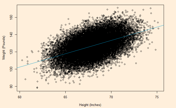
We will do a residual plot, a collection of points corresponding to the distances from the best-fit line.
H_data$resid <- resid(model)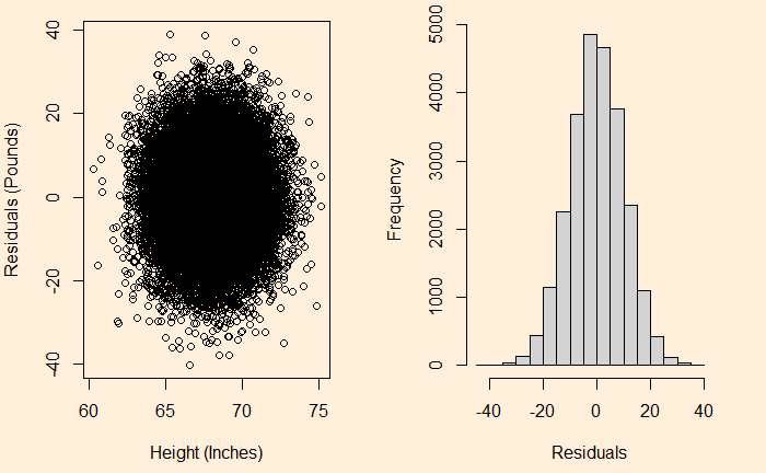
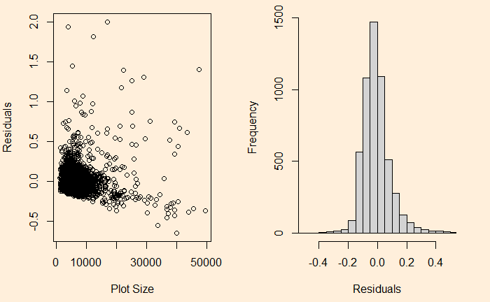
On the other hand, see the plot of sale price vs property area.
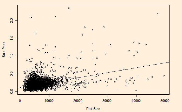
The relationship has heteroscedasticity, as evident from the skewness of residual towards one side.
Heteroskedasticity Read More »
White noise is a series that contains a collection of uncorrelated random variables. The following is a time series of Gaussian white noise generated as:
W_data <- 5*rnorm(500,0,1)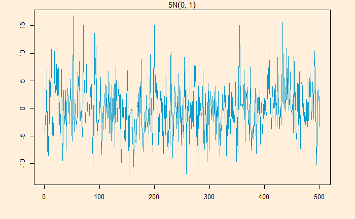
The series has zero mean and a finite variance.
Many real-life signals are composed of periodic signals contaminated by noise, such as the one shown above. Here is a periodic signal given by
2cos(2pi*t/100 + pi)
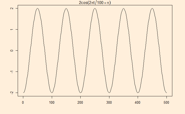
Now, add the white noise we developed earlier:

Data from a television production company suggests that 10% of their shows are blockbuster hits, 15% are moderate success, 50% do break even, and 25% lose money. Production managers select new shows based on how they fare in pilot episodes. The company has seen 95% of the blockbusters, 70% of moderate, 60% of breakeven and 20% of losers receive positive feedback.
Given the background,
1) How likely is a new pilot to get positive feedback?
2) What is the probability that a new series will be a blockbuster if the pilot gets positive feedback?
The first step is to list down all the marginal probabilities as given in the background.
| Pilot | Outcome | Total | |
| Positive | Negative | ||
| Huge Success | 0.10 | ||
| Moderate | 0.15 | ||
| Break Even | 0.50 | ||
| Loser | 0.25 | ||
| Total | 1.0 |
The next step is to estimate the joint probabilities of pilot success in each category.
95% of blockbusters get positive feedback = 0.95 x 0.1 = 0.095.
Let’s fill the respective cells with joint probabilities.
| Pilot | Outcome | Total | |
| Positive | Negative | ||
| Huge Success | 0.095 | 0.005 | 0.10 |
| Moderate | 0.105 | 0.045 | 0.15 |
| Break Even | 0.30 | 0.20 | 0.50 |
| Loser | 0.05 | 0.20 | 0.25 |
| Total | 0.55 | 0.45 | 1.0 |
The rest is straightforward.
The answer to the first question: the chance of positive feedback = sum of all probabilities under positive = 0.55 or 55%.
The second quesiton is P(success|positive) = 0.095/0.55 = 0.17 = 17%
| Pilot | Outcome | |
| P(Positive) | P(success|Positive) | |
| Huge Success | 0.095 | 0.17 |
| Moderate | 0.105 | 0.19 |
| Break Even | 0.30 | 0.55 |
| Loser | 0.05 | 0.09 |
| Total | 0.55 | 1.0 |
Basic probability: zedstatistics
Here, we plot the daily electricity production data that was used in the last post.

Following is the R code, which uses the filter function for building the 2-sided moving average. The subsequent plot represents the method on the first five points (the red circle represents the centred average of the first five points).
E_data$ma5 <- stats::filter(E_data$IPG2211A2N, filter = rep(1/5, 5), sides = 2)
For the one-sided:
E_data$ma5 <- stats::filter(E_data$IPG2211A2N, filter = rep(1/5, 5), sides = 1)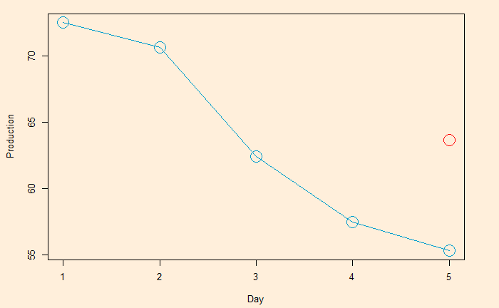
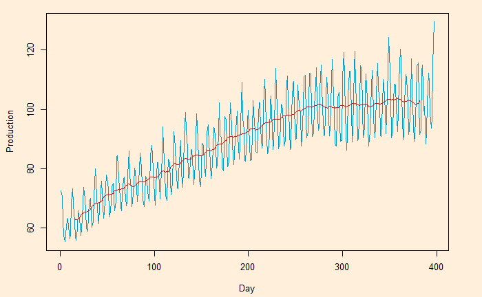
The 5-day moving average is below.

You can get a super-smooth data trend using the monthly (30-day) moving average.
Moving Average – Continued Read More »
Moving averages and means to smoothen noisy (time series) data, unearthing the underlying trends. The process is also known as filtering the data.
Moving averages (MA) are a series of averages estimated on a pre-defined number of consecutive data. For example, MA5 contains the set of all the averages of 5 successive members of the original series. The following relationship represents how a centred or two-sided moving average is estimated.
MA5 = (Xt-2 + Xt-1 + Xt + Xt+1 + Xt+2)/5
‘t’ represents the time at which the moving average is estimated. t-1 is the observation just before t, and t+1 means one observation immediately after t. To illustrate the concept, we develop the following table representing consecutive 10 points (electric signals) in a dataset.
| Date | Signal |
| 1 | 72.5052 |
| 2 | 70.6720 |
| 3 | 62.4502 |
| 4 | 57.4714 |
| 5 | 55.3151 |
| 6 | 58.0904 |
| 7 | 62.6202 |
| 8 | 63.2485 |
| 9 | 60.5846 |
| 10 | 56.3154 |
The centred MA starts from point 3 (the midpoint of 1, 2, 3, 4, 5). The value at 3 is the mean of the first five points (72.5052 + 70.6720 + 62.4502 + 57.4714 + 55.3151) /5 = 63.68278.
| Date | Signal | Average |
| 1 | 72.5052 | |
| 2 | 70.6720 | |
| 3 | 62.4502 | 63.68278 |
| 4 | 57.4714 | |
| 5 | 55.3151 | |
| 6 | 58.0904 | |
| 7 | 62.6202 | |
| 8 | 63.2485 | |
| 9 | 60.5846 | |
| 10 | 56.3154 |
This process is continued – MA on point 4 is the mean of points 2, 3, 4, 5 and 6, etc.
| Date | Signal | MA |
| 1 | 72.5052 | |
| 2 | 70.6720 | |
| 3 | 62.4502 | 63.68278 [1-5] |
| 4 | 57.4714 | 60.79982 [2-6] |
| 5 | 55.3151 | 59.18946 [3-7] |
| 6 | 58.0904 | 59.34912 [4-8] |
| 7 | 62.6202 | 59.97176 [5-9] |
| 8 | 63.2485 | 60.17182 [6-10] |
| 9 | 60.5846 | |
| 10 | 56.3154 |
The one-sided moving average is different. It estimates MA at the end of the interval.
MA5 = (Xt-4 + Xt-3 + Xt-2 + Xt-1 + Xt)/5
| Date | Signal | MA |
| 1 | 72.5052 | |
| 2 | 70.6720 | |
| 3 | 62.4502 | |
| 4 | 57.4714 | |
| 5 | 55.3151 | 63.68278 [1-5] |
| 6 | 58.0904 | 60.79982 [2-6] |
| 7 | 62.6202 | 59.18946 [3-7] |
| 8 | 63.2485 | 59.34912 [4-8] |
| 9 | 60.5846 | 59.97176 [5-9] |
| 10 | 56.3154 | 60.17182 [6-10] |
We will look at the impact of moving averages in the next post.
Continuing from the previous post, we have seen the variance inflation factor (VIF) of three variables in a database:
   pcFAT   Weight Activity
3.204397 3.240334 1.026226
The following is the correlation matrix of the three variables. You can see a reasonable correlation between the percentage of fat and weight.
               pcFAT     Weight    Activity
pcFAT     1.00000000  0.8267145 -0.02252742
Weight    0.82671454  1.0000000 -0.10766796
Activity -0.02252742 -0.1076680  1.00000000
Now, we create a new variable, FAT (in kg), multiplying fat percentage with weight. First, we rerun the correlation to check how the new variables relate.
MM_data <- M_data %>% select(pcFAT, Weight, Activity, FAT)
cor(MM_data)
pcFAT Weight Activity FAT
pcFAT 1.00000000 0.8267145 -0.02252742 0.9244814
Weight 0.82671454 1.0000000 -0.10766796 0.9684322
Activity -0.02252742 -0.1076680 1.00000000 -0.0966596
FAT 0.92448136 0.9684322 -0.09665960 1.0000000FAT, as expected, has a very high correlation with weight and fat percentage. Now, we run the VIF function on it.
model <- lm(BMD_FemNeck ~ pcFAT + Weight + Activity + FAT , data=M_data)
VIF(model)
pcFAT Weight Activity FAT
14.931555 33.948375 1.053005 75.059251
VIFs of those three variables are high.
Variance Inflation Factor Continued Read More »
We have seen estimating the variance inflation factor (VIF) is a way of detecting multicollinearity during regression. This time, we will work out one example using the data frame from “Statistics by Jim”. We will use R programs to execute the regressions.
This regression will model the relationship between the dependent variable (Y), the bone mineral density of the femoral neck, and three independent variables (Xs): physical activity, body fat percentage, and weight. The first few lines of the data are below:
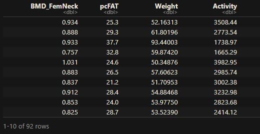
The objective of the regression is to find the best (linear) model that fits BMD_FemNeck with pcFAT, Weight, and Activity.
model <- lm(BMD_FemNeck ~ pcFAT + Weight + Activity, data=M_data)
summary(model)
Call:
lm(formula = BMD_FemNeck ~ pcFAT + Weight + Activity, data = M_data)
Residuals:
Min 1Q Median 3Q Max
-0.210260 -0.041555 -0.002586 0.035086 0.213329
Coefficients:
Estimate Std. Error t value Pr(>|t|)
(Intercept) 5.214e-01 3.830e-02 13.614 < 2e-16 ***
pcFAT -4.923e-03 1.971e-03 -2.498 0.014361 *
Weight 6.608e-03 9.174e-04 7.203 1.91e-10 ***
Activity 2.574e-05 7.479e-06 3.442 0.000887 ***
---
Signif. codes: 0 ‘***’ 0.001 ‘**’ 0.01 ‘*’ 0.05 ‘.’ 0.1 ‘ ’ 1
Residual standard error: 0.07342 on 88 degrees of freedom
Multiple R-squared: 0.5201, Adjusted R-squared: 0.5037
F-statistic: 31.79 on 3 and 88 DF, p-value: 5.138e-14The relationship will be:
5.214e-01 – 4.923e-03 x pcFAT + 6.608e-03 x Weight + 2.574e-05 x Activity
To estimate each VIF value, we will first consider the corresponding X value as the dependent variable (against the remaining Xs as the independent variables), do regression and evaluate the R-squared.
body fat percentage (pcFAT)
summary(lm(pcFAT ~ Weight + Activity , data=M_data))Call:
lm(formula = pcFAT ~ Weight + Activity, data = M_data)
Residuals:
Min 1Q Median 3Q Max
-7.278 -2.643 -0.650 2.577 11.421
Coefficients:
Estimate Std. Error t value Pr(>|t|)
(Intercept) 6.5936609 1.9374973 3.403 0.001 **
Weight 0.3859982 0.0275680 14.002 <2e-16 ***
Activity 0.0004510 0.0003993 1.129 0.262
---
Signif. codes: 0 ‘***’ 0.001 ‘**’ 0.01 ‘*’ 0.05 ‘.’ 0.1 ‘ ’ 1
Residual standard error: 3.948 on 89 degrees of freedom
Multiple R-squared: 0.6879, Adjusted R-squared: 0.6809
F-statistic: 98.1 on 2 and 89 DF, p-value: < 2.2e-16The R-squared is 0.6879, and the VIF for pcFAT is:
1/(1-0.6879) = 3.204101
weight (Weight )
summary(lm(Weight ~ pcFAT + Activity , data=M_data))Call:
lm(formula = Weight ~ pcFAT + Activity, data = M_data)
Residuals:
Min 1Q Median 3Q Max
-26.9514 -5.1452 -0.5356 5.1606 24.0891
Coefficients:
Estimate Std. Error t value Pr(>|t|)
(Intercept) 6.3369837 4.3740142 1.449 0.151
pcFAT 1.7817966 0.1272561 14.002 <2e-16 ***
Activity -0.0012905 0.0008532 -1.513 0.134
---
Signif. codes: 0 ‘***’ 0.001 ‘**’ 0.01 ‘*’ 0.05 ‘.’ 0.1 ‘ ’ 1
Residual standard error: 8.482 on 89 degrees of freedom
Multiple R-squared: 0.6914, Adjusted R-squared: 0.6845
F-statistic: 99.69 on 2 and 89 DF, p-value: < 2.2e-16The R-squared is 0.6914, and the VIF for Weight is 1/(1-0.6914) = 3.240441
physical activity (Activity)
summary(lm(Activity ~ Weight + pcFAT, data=M_data))Call:
lm(formula = Activity ~ Weight + pcFAT, data = M_data)
Residuals:
Min 1Q Median 3Q Max
-1532.8 -758.9 -168.0 442.6 4648.7
Coefficients:
Estimate Std. Error t value Pr(>|t|)
(Intercept) 2714.42 460.34 5.897 6.56e-08 ***
Weight -19.42 12.84 -1.513 0.134
pcFAT 31.33 27.74 1.129 0.262
---
Signif. codes: 0 ‘***’ 0.001 ‘**’ 0.01 ‘*’ 0.05 ‘.’ 0.1 ‘ ’ 1
Residual standard error: 1041 on 89 degrees of freedom
Multiple R-squared: 0.02556, Adjusted R-squared: 0.003658
F-statistic: 1.167 on 2 and 89 DF, p-value: 0.316
1/(1-0.02556) = 1.02623
The calculations can be simplified using the function VIF in ‘regclass’ package.
model <- lm(BMD_FemNeck ~ pcFAT + Weight + Activity, data=M_data)
VIF(model)
pcFAT Weight Activity
3.204397 3.240334 1.026226 All three VIF values remain reasonably low (< 10); therefore, we don’t suspect collinearity in these three variables.
Detecting Multicollinearity – VIF Read More »
The first thing that can be done is to find pairwise correlations between all X variables. If two variables are perfectly uncorrelated, the correlation is zero, one suggesting a perfect correlation. In our case, a correlation of > 0.9 must sound an alarm for multicollinearity.
Another method to detect multicollinearity is the Variance Inflation Factor (VIF). VIF estimates how much the variance of the estimated regression coefficients is inflated compared to when Xs are not linearly related. The way to estimate VIF work the following way:
Detecting Multicollinearity Read More »
Regression, as we know, is the description of the dependent variable, Y, as a function of a bunch of independent variables, X1, X2, X3, etc.
Y = A0 + A1 X1 + A2 X2 + A3 X3 + …
A1, A2, etc., are coefficients representing the marginal effect of the respective X variable on the impact of Y while keeping all the other Xs constant.
But what happens when the X variables are correlated? – that is multicollinearity.
Regression – Multicollinearity Read More »