Here is another problem with conditional probability. There are three men and two women. If one of the men is a carpenter, what is the probability of randomly selecting a carpenter and a man from the group?
Let M represent man, W represents woman, and C represents carpenter. P(M AND C) = P(M) x P(C|M) The probability of choosing a man is 3 in 5; the probability that it’s a carpenter, given a man is chosen, is 1/3 = 3/5 x 1/3 = 1/5
This can also be done the following way P(C AND M) = P(C) x P(M|C) The probability of choosing a man is 1 in 5; the probability that it’s a man, given it’s a carpenter, is 100%. = 1/5 x 1 = 1/5
There are three fair 6-sided dice with the following sides: A. [2, 2, 4, 4, 9, 9] B. [1, 1, 6, 6, 8, 8] C. [3, 3, 5, 5, 7, 7]
If A plays against B, what is the probability of A winning?
A vs B The required Probability is: Probability of rolling a 2 x probability of 2 winning + Probability of rolling a 4 x probability of 4 winning + Probability of rolling a 9 x probability of 9 winning = (2/6) x (2/6) + (2/6) x (2/6) + (2/6) x 1 = 20/36 = 55.55%
Count the number of red dots and divide it by the total number of dots.
What is the chance of B winning if B plays against C?
B vs C = (2/6) x (0) + (2/6) x (4/6) + (2/6) x 1 = 20/36 = 55.55%
and
C vs A = (2/6) x (2/6) + (2/6) x (4/6) + (2/6) x (4/6)= 20/36 = 55.55%
Each die beats the other with a probability of 55.55%.
1 in 10 sets of twins are identical, and 9 in 10 are fraternal. What is the probability that Adam and his twin brother Ben are identical twins?
Fraternal twins result from fertilising two eggs with two sperm during the same pregnancy. They may not be the same sex. On the other hand, identical twins result from the fertilisation of a single egg by a single sperm, with the fertilised egg then splitting into two. As a result, identical twins share the same genomes and are always of the same sex.
National Human Genome Reseach Institute
Contrary to how it appears otherwise, this is not a marginal probability but a conditional. The information that the twins are both males (Adam and his brother) triggers this shift. We will use the Bayes rule to solve this problem. The probability that Adam and Ben are identical twins, given they are males, is: P(I|M) = P(M|I)xP(I)/[P(M|I)xP(I) + P(M|F)xP(F)]
P(M|I) = Probability of both males, given they are identical twins, is 1/2 (always same sex). P(I) = Probability of twins being identical twins = 1/10 P(M|F) = Probability of both males, given they are fraternal twins, is 1/4 (MM out of the possible four, MM, FM, MF, FF) P(F) = Probability of twins being fraternal twins = 9/10
People v. Collins was a 1968 trial in the Supreme Court of California that reversed the convictions of Janet and Malcolm Collins by a jury in Los Angeles of second-degree robbery. The events that led to the original conviction were as follows:
On June 18, 1964, Mrs. Juanita Brooks was walking home along an alley in San Pedro, City of Los Angeles. She was suddenly pushed to the ground, and she saw a young woman running, wearing “something dark.” She had hair “between a dark blond and a light blond,”. After the incident, Mrs Brooks discovered that her purse, containing between $35 and $40, was missing.
At about the same time, John Bass, who lived on the street at the end of the alley, saw a woman run out of the alley and enter a yellow automobile driven by a black male wearing a moustache and beard.
The prosecutor (of the jury trial) brought a statistician to prove the crime using the laws of probability. The expert hypothesised the following chances and made his calculations.
Characteristic
Probability
1
Yellow automobile
1/10
2
Man with moustache
1/4
3
Girl with poleytail
1/10
4
Girl with blondehair
Girl with blonde hair
5
Interracial couple in a car
1/10
6
Interracial couple in car
1/1000
The profession used the product rule (the AND rule) of probability to prove the case. Multiplying all the probabilities, he concluded that the chance for any couple to possess the characteristics of the defendants is 1/12,000,000! Note that such multiplication is only possible if the individual probabilities are independent.
But the statistician (and the jury) convenient ignored a few things: 1) The validity of the probabilities. Those were his ‘inventions’ without any support from data. 2) The events (characteristics) were not independent from each other. More likely than not, the person with a beard has a moustache. 3) Once, a blond girl and a black man with a beard were counted, talking about the low probability of an interracial couple in a car is wrong. Think about it—the probability of an interracial couple, given one is a blond girl and another is a bearded black man, must be close to 1.
References
People v. Collins: Justia US Law The Worst Math Ever Used In Court: Vsauce2 A Conversation About Collins: William B. Fairley; Frederick Mosteller
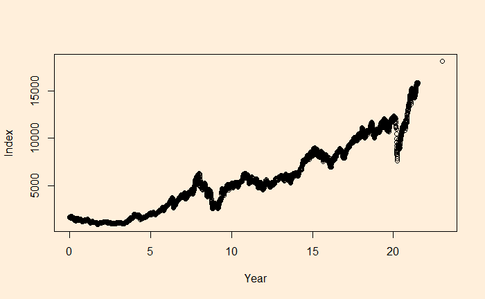
The world is experiencing another El Niño episode. El Niño is a climate pattern of more than usual warming surface waters in the eastern Pacific Ocean. It is defined as a phenomenon in the equatorial Pacific Ocean (Niño 3.4 region) marked by a positive departure for five consecutive three-month running mean sea surface temperature (SST = 28°C) by +0.5°C.
We have seen examples of regression where the basic assumption of uncorrelated residuals is compromised. Finding the autocorrelation of the residuals using Durbin–Watson is one way to diagnose the correlation. Here, we perform a step-by-step estimation.
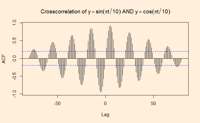
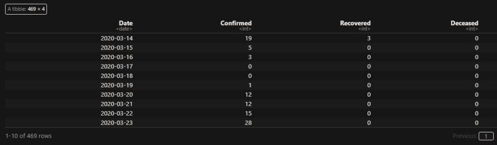
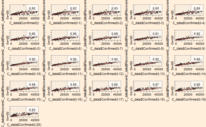
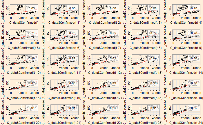
If autocorrelation represents the correlation of a variable with itself but at different time lags, cross-correlation is between two variables (at time lags). We will use a few R functions to illustrate the concept. The following are data from our COVID archives.
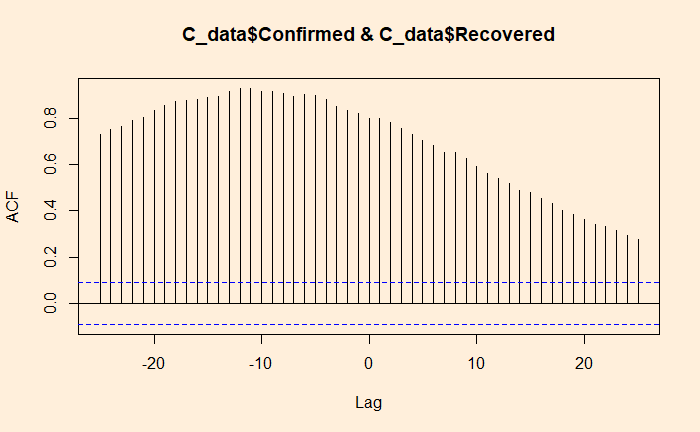
‘ccf’ function of ‘stats’ library is similar to ‘acf’ we used for the autocorrelation. Here is the cross-collation between the infected and the recovered.
ccf(C_data$Confirmed, C_data$Recovered, 25)
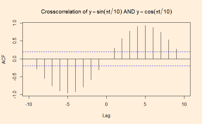
The ‘lag2.plot’ function of the ‘astsa’ library presents the same information differently.
lag2.plot(C_data$Confirmed, C_data$Recovered, 20)
The correlation peaked at a lag of about 12 days, which may be interpreted as the recovery time from the disease. On the other hand, the infected vs deceased gives a slightly higher lag at the maximum correlation.
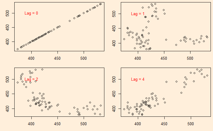
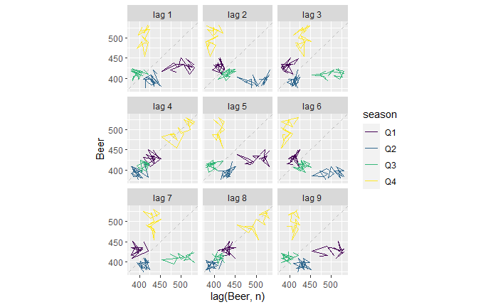
We continue from the Aus beer production data set. In the last post, we manually built scatter plots at a few lags (lag = 0, 1, 2, and 4) and introduced the ‘acf’ function.
There is another R function, ‘gg_lag’, which can be an even better illustration.
new_production %>% gg_lag(Beer)
For example, the lag = 1 plot (top left). The yellow cluster represents the plot of Q4 on the Y-axis against Q3 of the same year on the X-axis. On the other hand, the purple cluster represents the plot of Q1 on the Y-axis against Q4 of the previous year on the X-axis.
Similarly, for the lag = 2 plot (top middle), The yellow represents the plot of Q4 against Q2 (two quarters earlier) of the same year. The purple represents the plot of Q1 against Q3 of the previous year.
The lag = 4 plot shows a strong positive correlation (everyone on the diagonal line). This is not surprising; it plots Q4 of one year against Q4 of the previous year, Q1 of one year with Q1 of the previous year, etc.
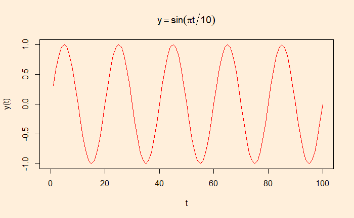
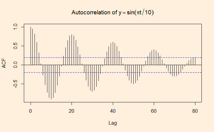
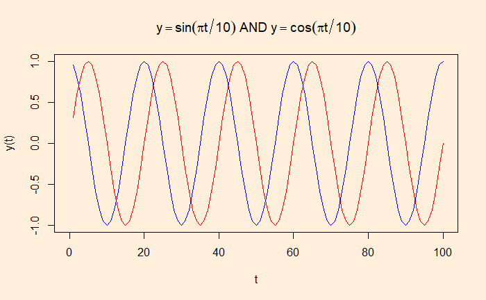
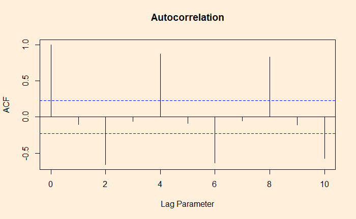
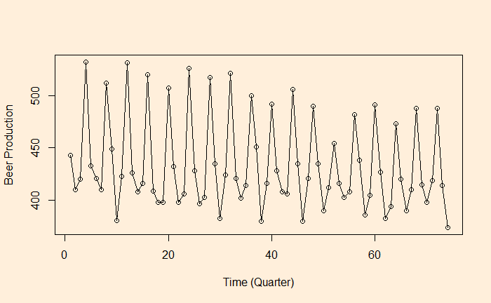
As we have seen, autocorrelation is the correlation of a variable in a time series with itself but at a time lag. For example, how are the variables at time ts correlated to the t-1s? We will use the aus_production dataset from the R library ‘fpp3’ to illustrate the concept of autocorrelation.
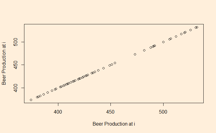
Let’s plot the production data with itself without any lag in time.
plot(B_data, B_data, xlab = "Beer Production at i", ylab = "Beer Production at i")
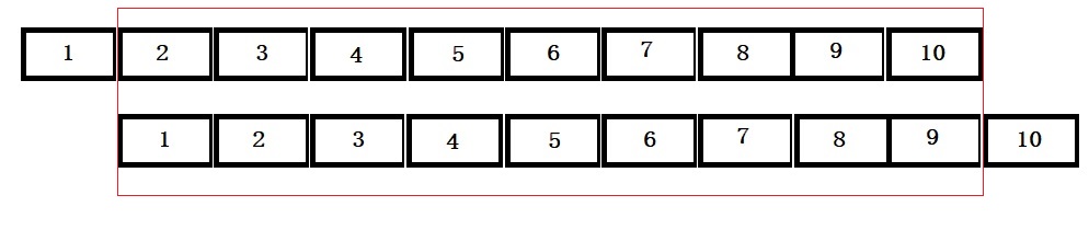
There is no surprise here; the data is in perfect correlation. In the next step, we will give a lag of one time interval, i.e., a plot of (2,1), (3,2), (4,3), etc. The easiest way to achieve this is to remove the first element of the vector and plot against the vector with the last element removed.
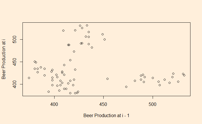
plot(B_data[-1], B_data[-n], xlab = "Beer Production at i - 1", ylab = "Beer Production at i")
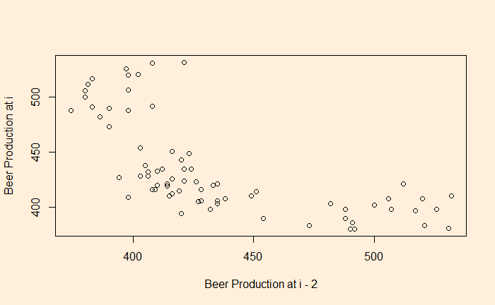
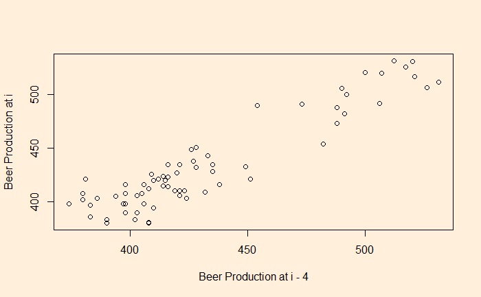
You clearly see a lack of correlation. What about a plot with a lag of 2 and 4?
There is a negative correlation compared with the time series 2 quarters ago.
There is a good correlation compared with the time series 4 quarters ago.
The whole process is established using the autocorrelation function (ACF).
ACF at large parameter 1 indicates how successive values of beer production relate to each other, 2 indicates how production two periods apart relate to each other, etc.