Goodness of Fit using tigerstats

We have seen how the R package ‘tigerstats’ can help visualise basic statistics. The library has several functions and datasets to teach statistics at an elementary level. We will see a couple of them that enable hypothesis testing.

chi-square test

We start with a test for Independence using the chi-square test. The example is the same as we used previously. Here, we create the database with the following summary.

High SchoolBachelorsMastersPh.d.Total
Female60544641201
Male40445357194
Total100989998395
as_tibble(educ)

The function to use is ‘chisqtestGC’, which takes two variables (~var1 + var2) to test their association. Additional attributes such as graph and verbose yield the relevant graph (ch-square curve) for the P-value and details of the output.

chisqtestGC(~EDU+SEX, data=educ, graph = TRUE, verbose = TRUE)
Pearson's Chi-squared test 

Observed Counts:
             SEX
EDU           Female Male
  Bachelors       54   44
  High School     60   40
  Masters         46   53
  Ph.d.           41   57

Counts Expected by Null:
             SEX
EDU           Female  Male
  Bachelors    49.87 48.13
  High School  50.89 49.11
  Masters      50.38 48.62
  Ph.d.        49.87 48.13

Contributions to the chi-square statistic:
             SEX
EDU           Female Male
  Bachelors     0.34 0.35
  High School   1.63 1.69
  Masters       0.38 0.39
  Ph.d.         1.58 1.63


Chi-Square Statistic = 8.0061 
Degrees of Freedom of the table = 3 
P-Value = 0.0459 

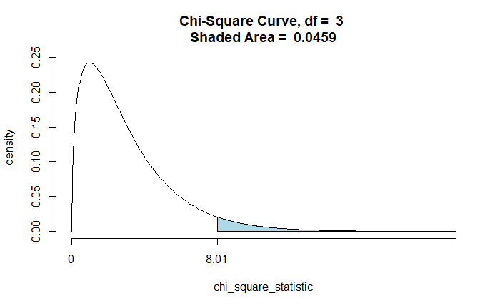
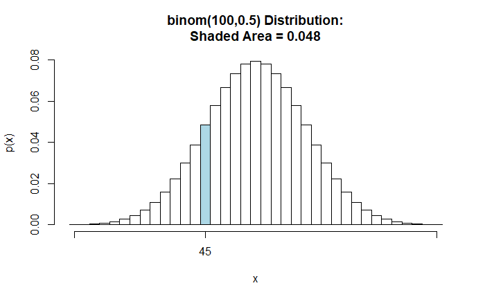
Binomial test for proportion

Suppose a coin toss landed on 40 heads in 100 attempts. Perform a two-sided hypothesis test for p = 0.5 as the Null.

binomtestGC(x=40,n=100,p=0.5, alternative = "two.sided", graph = TRUE, conf.level = 0.95)

x = variable under study
n = size of the sample
p = Null Hypothesis value for population proportion
alternative = takes “two.sided”, “less” or “greater” for the computation of the p-value.
conf.level = number between 0 and 1, indicating the confidence interval
graph = If TRUE, plot graph of p-value

Exact Binomial Procedures for a Single Proportion p:
	Results based on Summary Data

Descriptive Results:  40 successes in 100 trials

Inferential Results:

Estimate of p:	 0.4 
SE(p.hat):	 0.049 

95% Confidence Interval for p:

          lower.bound         upper.bound          
          0.303295            0.502791             

Test of Significance:

	H_0:  p = 0.5 
	H_a:  p != 0.5 

	P-value:		P = 0.0569 
binomtestGC(x=40,n=100,p=0.5, alternative = "less", graph = TRUE, conf.level = 0.95)
Exact Binomial Procedures for a Single Proportion p:
	Results based on Summary Data

Descriptive Results:  40 successes in 100 trials

Inferential Results:

Estimate of p:	 0.4 
SE(p.hat):	 0.049 

95% Confidence Interval for p:

          lower.bound         upper.bound          
          0.000000            0.487024             

Test of Significance:

	H_0:  p = 0.5 
	H_a:  p < 0.5 

	P-value:		P = 0.0284 

Goodness of Fit using tigerstats Read More »

Probability, Likelihood and tigerstats

This post refreshes the probability vs likelihood concept and presents a few R functions from the tigerstats library. As usual, we begin with a coin-flipping exercise. What is the probability of obtaining 45 heads upon flipping 100 fair coins? A fair coin is one in which the chance of getting heads equals the chance of getting tails: 0.5.

Here is a graphical representation of the ask.

library(tigerstats)
bound <- c(45,45)
pbinomGC(bound,region="between",size=100,prob=0.5,graph=TRUE)

Coin tossing is a discrete event, and the Y-axis represents the probability. The probability of obtaining 45 heads while flipping 100 fair coins is 0.048.

Now, consider a continuous distribution. Suppose the heights of adults are normally distributed in a population with a mean of 175 cm and a standard deviation of 6.5 cm. What is the probability that a random person measures height between 185 and 190 cm?

sample <- c(185,190)
pnormGC(bound=sample,region="between", mean=175,sd=6.5,graph=TRUE)

Notice a few things: the Y-axis is not probability but probability density. The required probability is the area (under the curve) between two values, the height between 185 and 190 cm = 0.0515. In a continuous distribution, where the probability can take every possible value between 0 and 1, getting the chance for precise height (say, 180.0000) does not make sense.

Likelihood

If probability was about getting 45 heads for a coin with p = 0.5 tossed 100 times, the likelihood is the mirror image of that. What is the likelihood of having a fair coin (p = 0.5) if the coin lands 45 heads in 100 tosses?

In likelihood discussions, you have the data, i.e., 45 heads in 100 tosses. The investigator’s task is to find out the coin bias.
The likelihood that it’s an unbiased coin (p = 0.5), given that 45 in 100 landed on heads, is 0.048.
The likelihood that the coin is biased with p = 0.55, given that 45 in 100 landed on heads, is 0.011.
The likelihood that the coin is biased p = 0.4, given that 45 in 100 landed on heads, is 0.048.

Similarly, for heights,
The likelihood of a distribution with mean = 175 cm and a standard deviation = 6.5 cm, given the measured height = 185, is 0.019
The likelihood of a distribution with mean = 180 cm and a standard deviation = 6.5 cm, given the measured height = 185, is 0.046

In summary

Probability is about the chance of data under a given distribution, P(Data|Distribution)

Likelihood is about the distribution for the given data, L(Distribution|Data)

Reference

Probability is not Likelihood. Find out why!!!: StatQuest with Josh Starmer

Probability, Likelihood and tigerstats Read More »

Screen Time and Happiness

The effect of screen time on mental and social well-being is a subject of great concern in child development studies. The common knowledge in the field revolves around the “dispalcement hypothesis”, which says that the harm is directly proportional to the exposure.

Przybylski and Weinstein published a study on this topic in Psychological Science in 2017. The research analysed data collected from 120,115 English adolescents. Mental well-being (the dependent variable) was estimated using the Warwick-Edinburgh Mental Well-Being Scale (WEMWBS ). The WEMWBS is a 14-item scale, each answered on a 1 to 5 scale, ranging from “none of the time” to “all the time.” The fourteen items in WEMWBS are:

1I’ve been feeling optimistic about the future
2I’ve been feeling useful
3I’ve been feeling relaxed
4I’ve been feeling interested in other people
5I’ve had energy to spare
6I’ve been dealing with problems
7I’ve been thinking clearly
8I’ve been feeling good about myself
9I’ve been feeling close to other people
10I’ve been feeling confident
11I’ve been able to make up my own mind about things
12I’ve been feeling love
13I’ve been interested in new things
14I’ve been feeling cheerful

The study results

I must say, the authors were not alarmists in their conclusions. The study showed a non-linear relationship between screen time and mental well-being. Well-being increased a bit with screen time but later declined. Yet, the plots were in the following form (see the original paper in the reference for the exact graph).

A casual look at the graph shows a steady decline in mental well-being as the screen time increases from 2 hours onwards. Until you notice the scale of the Y-axis!

In a 14-item survey with a 1-5 range in scale, the overall score must range from 14 (min) to 70 (max). Instead, In the present plot, the scale was from 40 to 50, thus visually exaggerating the impact. Had it been plotted following the (unwritten) rules of visualisation, it would have looked like this:

To conclude

Screen time impacts the mental well-being of adolescents. It increases a bit, followed by a decline. The magnitude of the decrease (from 0 screen time to 7 hr) is about 3 points on a 14-70 point scale.

References

Andrew K. Przybylski and Netta Weinstein, A Large-Scale Test of the Goldilocks Hypothesis: Quantifying the Relations between Digital-Screen Use and the Mental Well-Being of Adolescents, Psychological Science, 2017, Vol. 28(2) 204–215.
Joshua Marmara, Daniel Zarate, Jeremy Vassallo, Rhiannon Patten, and Vasileios Stavropoulos, Warwick Edinburgh Mental Well-Being Scale (WEMWBS): measurement invariance across genders and item response theory examination, BMC Psychol. 2022; 10: 31.

Screen Time and Happiness Read More »

Generalised Linear Models

In an ordinary linear model, like linear regression exercises, we express the dependant variation (y) as a function of the independent variable (x) as:

y_i = \beta_0 + \beta_1 x_i + \epsilon_i

The equation is divided into two parts. The first part is the equation of a line.

\mu_i = \beta_0 + \beta_1 x_i

where beta0 is the intercept and beta1 is the slope of the line. It just described the line (the approximation), but you need to add the error term to include the points around the line. The second part is the error term or the points around the idealised line.

\epsilon_i = N(\mu_i, sd)

The points around the line are normally distributed in linear regression, so the epsilon term is normal.

LM to GLM

Imagine if the dependent variable is binary—it takes one or zero. The random component (error term) is no longer normally distributed in such cases. That is where the concept of generalised linear models (GLM) comes in. Here, the first part remains the same, while the second part can take other types of distributions as well. In the case of binary, as in logistic regression, GLM is used with binomial distribution through a link function.

\eta = \beta_0 + \beta_1 x

link function

\eta = logit(\mu)

random component is a binomial error distribution family.

\epsilon_i = Binomial(\mu)

In Poisson regression, the error term takes a Poisson distribution.

\eta = \beta_0 + \beta_1 x

\eta = log(\mu)

\epsilon_i = Poisson(\mu)

In R, you use glm() with an attribute on the family as, glm(formula, family = “binomial”)

binomial()
Family: binomial 
Link function: logit 
poisson()
Family: poisson 
Link function: log 

Generalised Linear Models Read More »

Poisson Regression 

We have seen the use of linear regression models for continuous variables and logistic regression for binary variables. Another class of variables is called count variables, such as,

The number of claims received per month by an insurance company
Weekly accidents happening in a particular region

The dependent variables (claims or accidents) in these examples have a few standard features. The data represent numbers (counts) or rates (counts per time). They also can only take values of zero or positive discrete numbers. As the Poisson random variable is used to model counts, the relevant regression in the above examples could be Poisson regression.

Poisson Regression  Read More »

Flight Accidents

YearAccidents
197624
197725
197831
197931
198022
198121
198226
198320
198416
198522

We assume that flight accidents are random and independent. This implies that the likelihood function (the nature of the phenomenon) is likely to follow a Poisson distribution. Let Y be the number of events occurring within the time interval.

Y|\theta = Pois(\theta)

Theta is the (unknown) parameter of interest, and y is the data (total of 10 observations). We will use Bayes’ theorem to estimate the posterior distribution p(theta|data) from a prior, p(theta). As we established long ago, we select gamma distribution for the prior (conjugate pair of Poisson).

Flight Accidents Read More »

Bland-Altman Plot

Bland-Altman analysis is used to study the agreement between two measurements. Here is how it is created.

Step 1: Collect the two measurements

Sample_Data <- data.frame(A=c(6, 5, 3, 5, 6, 6, 5, 4, 7, 8, 9,
10, 11, 13, 10, 4, 15, 8, 22, 5), B=c(5, 4, 3, 5, 5, 6, 8, 6, 4, 7, 7, 11, 13, 5, 10, 11, 14, 8, 9, 4))

Step 2: Calculate the means of the measurement 1 and measurement 2

Sample_Data$average <- rowMeans(Sample_Data) 

Step 3: Calculate the difference between measurement 1 and measurement 2

Sample_Data$difference <- Sample_Data$A - Sample_Data$B

Step 4: Calculate the limits of the agreement based on the chosen confidence interval

mean_difference <- mean(Sample_Data$difference)
lower_limit <- mean_difference - 1.96*sd( Sample_Data$difference )
upper_limit <- mean_difference + 1.96*sd( Sample_Data$difference )

Step 5: Create a scatter plot with the mean on the X-axis and the difference on the Y-axis. Mark the limits and the mean of difference.

ggplot(Sample_Data, aes(x = average, y = difference)) +
  geom_point(size=3) +
  geom_hline(yintercept = mean_difference, color= "red", lwd=1.5) +
  geom_hline(yintercept = lower_limit, color = "green", lwd=1.5) +
  geom_hline(yintercept = upper_limit, color = "green", lwd=1.5) +
  ggtitle("")+ 
       ylab("Difference")+
       xlab("Average") 

Bland-Altman Plot Read More »

Larry Bird and Binomial Distribution

Following are the free throw statistics from basketball great Larry Bird’s two seasons.

Total pairs of throws: 338
Pairs where both throws missed: 5
Pairs where one missed: 82
Pairs where both made: 251

Test the hypothesis that Mr Bird’s free throw follows binomial distribution with p = 0.8.
H0 = Bird’s free throw probability of success followed a binomial distribution with p = 0.8
HA = The distribution did not follow a binomial distribution with p = 0.8

We will use chi-square Goodness of Fit to test the hypothesis. The probabilities of making 0, 1 and 2 free throws for a person with a probability of success of 0.8 is

bino_prob <- dbinom(0:2, 2, 0.8)
 0.04 0.32 0.64

The chi-square test is:

chisq.test(child_perHouse, p = bino_prob, rescale.p = TRUE)

	Chi-squared test for given probabilities

data:  child_perHouse
X-squared = 17.256, df = 2, p-value = 0.000179

Larry Bird and Binomial Distribution Read More »

This Sentence is False!

‘This sentence is false’ is an example of what is known as the Liar Paradox.

This sentence is false.

Look at the first option for the answer—true. To do that, we check what the sentence says about itself. It says about itself that it is false. If it is true, then it is false, which is a contradiction, and therefore, the answer ‘true’ is not acceptable.

The second option is false. Since the sentence claims about itself as false, then it’s false that it’s false, which again is a contradiction.

This Sentence is False! Read More »