July 2024

Fallacy of Equivocation

A fallacy is a bad argument mistaken for a good one. A famous example of a fallacy is:
1. Computers are products of intelligent design.
2. The human brain is a computer.
Therefore, the human brain is a product of intelligent design.

It is easy to confuse the above argument with the following valid argument.
1. All A’s are B
2. x is an A
Therefore, x is B

So what is wrong with the brain-computer argument, which was right for the A-B? In the A-B statement, A and B must mean the same thing in both arguments. But in the brain-computer case, the term computer has different meanings in two premises. In the second premise (“the human brain is a computer”), the word computer is used broadly – as a system that performs computations.

It is equivocation, i.e., employing two different things by the same name. In the brain-computer argument, we equivocated the word computer to represent two different things that are broadly similar in two premises. In the first premise, the word computer means specifically artificial computers humans built. However, in the second premise, the word was used broadly as an information processing system.

Reference

The Small Sample Fallacy: Kevin deLaplante

Fallacy of Equivocation Read More »
The Small Sample Fallacy

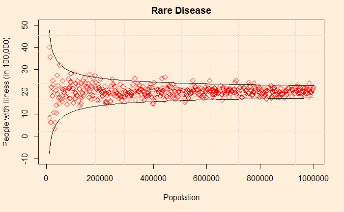
You may remember an older post titled “Life in a Funnel“. It discussed the wired (i.e., extreme) variation of averages (of the rate of certain illnesses, income levels, etc.) arising from groups and places with smaller populations. An often-quoted example is the prevalence of the lowest rates of kidney cancer in the US. These are regions of often rural, sparsely populated, traditionally Republican states. People who come across this data would rationalise this to cleaner air, healthier lifestyles or fresh foods. But when it comes to regions with the highest prevalence of the same disease, they also belong to mostly rural, less populated, Republican!

The incidence of disease is enclosed in a 95% confidence interval.

The plot shows the variability of observed averages simulated from precisely the same incident rate. As the sample size decreases, the sample average goes up or down dramatically, creating an illusion that forces the public to believe something real. This is known as the small sample fallacy. It’s a mistake where one attaches a causal explanation to a statistical artefact due to a smaller sample size.

A simple illustration is to imagine a bowl containing several marbles – 50% red and 50% green. If you take only four samples out of it to check the proportion, there is a 12.5% chance of getting either all green or all red. Work out this binomial probability with p = 0.5, n = 4 and x = 4.
P(X=4 red) = 4C4 0.54 0.50 = 0.0625
P(X=4 green) = 4C4 0.54 0.50 = 0.0625
P(all red or all green) = 0.0625 + 0.0625 = 0.125 or 12.5%.

There is a 12.5% chance of seeing an extreme sample average from an otherwise perfectly balanced population. In other words, 12 investigators out of 100 will see a distorted value!

Now, increase the samples to 10, the probability of observing all red or all green reduces dramatically to,
P(all red or all green) = 10C10 0.5100.50 + 10C10 0.5100.50
P(all red or all green) = 0.00098 + 0.00098 = 0.00196 or just 0.2%.

Reference

The Small Sample Fallacy: Kevin deLaplante

The Small Sample Fallacy Read More »

Prisoner’s Envelope

Professor Hugo F. Sonnenschein of the University of Chicago explains the famous prisoner’s dilemma differently.

There are two players, A and B, and a moderator. The moderator hands A and B a dollar each and an envelope. Players can keep the dollar in their pocket or leave it inside the envelope. Players then return the envelope to the moderator; the moderator can’t see what each has done. The moderator then looks at the envelopes and doubles the amount she sees inside them. In other words, if she sees a dollar inside the envelope, she makes it two; she doesn’t add anything if she sees nothing.

The moderator then switches the envelopes (envelope A to B and B to A) and gives them back to the players. What is the best strategy for the players to do in the first place—keep the dollar inside the envelope or hold it with them?

Player A can do two things with four possible outcomes; one guarantees a profit.

Keep the dollar in the pocket and return an empty envelope. This guarantees $1 if the other player does the same, or A gets two more dollars if player B is magnanimous (returning her envelope with a dollar in it).

The second option for player A is to return the envelope with one dollar in it. Again, there are two possible outcomes: A gets nothing if player B follows A’s first strategy (keeping a dollar in her pocket) or two if the other returns with a dollar in the envelope.

If you want to be formal with the payoff matrix, here it is.

While it is perfectly understandable that corporation (by each putting their dollars inside the envelope) brings prosperity to both (2 dollars each), the game theory doesn’t work that way. It will give you a strategy that guarantees you a profit irrespective of what the other person would do. In other words, the rational approach is to be selfish.

Game Theory and Negotiation: Becker Friedman Institute University of Chicago

Prisoner’s Envelope Read More »

Gambler’s Ruin

A gambler starts with a fixed amount of money ($i) and bets $1 in a fair game (i.e., the probability of winning or losing is 0.5) each time until she has 0 or n dollars. What is the probability she ends up with $0, and what chance does she get $n?

This is a perfect example of a Markov process. This is because the only thing relevant to the gambler at any point in time is the money she has at that time. Imagine her end goal is to reach 5. Let’s assume she has p chance to win a dollar and q = 1-p chance to lose the bet amount. The Markov chain representation is as follows.

Here is the translation matrix.

Take two cases: a fair bet (p = 0.5, q = 0.5) and a favourable bet (p = 0.6, q = 0.4). She starts with $3, represented as X = [0, 0, 0, 1, 0, 0]. Note that the first element represents 0, then 1, etc, and the sixth element denotes 5 (the goal). After 50 steps, the end state probability is,
P50 * X

P50 * [0, 0, 0, 1, 0, 0] = [0.4, 0, 0, 0, 0, 0.6]. The answer has to be the fourth column of P50. There is a 40% chance she ends up 0 and a 60% chance it’s 5$.

By the way, for p = 0.5, the analytical solution for the probability of reaching n, starting from i, is,
ai = i/n; a3 = 3/5 = 60%.

For p does not equal 0.5, it is,

ai = (1 – ri)/(1 – rn)
r = (1-p)/p

Now, imagine the probability of winning is 0.6.

p = 0.6; r = 0.4/0.6 = 0.67
a3 = (1 – r3)/(1 – r5) = 0.81
See the fourth column of the matrix above.

L26.9 Gambler’s Ruin: MIT OpenCourseWare

Gambler’s Ruin Read More »

Markovian Umbrella Run

Becky has four umbrellas. During her workday, she travels between home and the office. She takes an umbrella only when it rains; otherwise, it remains where it was last—in the office or at home. Suppose on a given day that all her umbrellas are in the office, whereas she’s at home preparing for the office, and if it rains, she will get wet. The question is:
If the location has a 60% probability of rain, what is the chance that Becky gets wet?

The problem can be solved as a Markovian chain. For that, we must divide the conditions into five states. They are
0: no umbrella state
1: one umbrella
2: two umbrellas
3: three umbrellas
4: four umbrellas

We must know what movements are possible from one state to another to develop translation probabilities.

From 0: Becky must go from 0 to 4, from one place without an umbrella to the other with all umbrellas. As this must happen irrespective of whether it rains or not, the probability of this movement is 1.

From 1: If it rains, p = 0.6, Becky carries the umbrella with her. In other words, she goes from state 1 to state 4 (3 already + 1 incoming).
If it doesn’t rain, p = 0.4, she will go from state 1 to state 3.

From 2: If it rains, state 2 to state 3. If it doesn’t rain, she will go from 2 to 2.

From 3: If it rains, 3 to 2; if it doesn’t, 3 to 1.

From 4: If it rains, 4 to 1; if it doesn’t, 4 to 0.

Here is the diagram representing the chain.

The translation matrix is

The required task is to find the stable end distribution of cities, which can be done using the relationship.

Xn = Pn X0

We use the Matrix calculator for P100

Multiply this with any starting distribution, we get the end state probabilities as,

The probability that she’s at state 0, P(0) = 0.09. Since the probability of rain when Becky is at 0 state is 0.6, the chance she gets drenched is 0.09 x 0.6 = 0.054 or about 5%.

Markovian Umbrella Run Read More »

Confidence Interval in Poll Surveys

Consider a large population from which you are randomly sampling 1000 people. The ask is to get a simple YES or NO answer from each survey participant about a candidate. Suppose 450 people gave a YES answer; what is the margin of error in the estimate if you use a confidence level of 95%?

h \pm 1.96 . \frac{\sigma} {\sqrt{n}}

The sample size, n = 1000. Since 450 out of 1000 responded YES, we approximate the value 450/1000 (the sample ratio, h) as the population probability (p) for YES. The next step is to estimate sigma, the standard deviation. This can be done in two ways.

Solution as Bernoulli trial

This is a Bernoulli trial, and the standard deviation per trial is nothing but the square root of p x (1-p), where p is the probability of YES.
sd = root(p x (1-p) = root(0.45 x 0.55) = 0.497.

\\ 0.45 \pm 1.96 . \frac{0.497} {\sqrt{1000}} \\\\ 0.45 \pm 0.031

Thus, the population percentage p is in the interval [0.45 – 0.031, 0.45 + 0.031] or [0.42, 0.48] at 95% confidence interval.

Confidence Interval in Poll Surveys Read More »

Polls and 3.5%

In this post and the next, we will do the poll survey problem in two different ways. First, what number of candidates is required in the survey to form a signal of a 3.5 percentage point difference?

The steps are
find the signal (we know that already (3.5% or 0.035)
find the noise (standard deviation)
estimate signal/nose and equate it to 1.96/root(n)
estimate n

Standard deviation

Imagine a survey asking a random potential voter a question about a candidate. The answer is YES or NO. YES carries 1, and NO carries 0 value. Let p be the probability of getting a YES, something we don’t know now. From Bernaulli trial (this can be a decent Bernaulli trial), the standard deviation is p x (1-p) per trial. For p = 0.5 (equal probabilities for YES and NO), the standard deviation (sd) is 0.5. The value for sd is 0.49 for 60:40 and 40:60, 0.46 for 70:30 and 30:70 etc. Therefore, using a standard deviation of 0.5 in the poll won’t be a big crime.

Samples

signal/noise = 0.035/0.5 = 0.07
n = (1.96/0.07)2
= 780
or about 1000 people.

We will address the same problem in the opposite way in the next post.

Polls and 3.5% Read More »

Confidence with an Edge

Anne has developed a 3% edge in sports betting based on some intelligent math, but she has yet to learn the exact advantage. She wants to bet $ 1 on a team at odds of 1/2. How many bets does she need to make before she knows her edge?

Before we get into the question, let’s familiarise ourselves with what Nate Silver popularised as ‘signal’ and ‘noise’. The signal is what we expect—in simple language, it’s the mean. The noise is the variability, or, in other words, the standard deviation.

The problem mentioned above is another way of stating the number of trials required for Anne to develop the confidence interval (say 95%) that can clearly distinguish the signal (the edge, 0.03) from the noise (the standard deviation). Just a reminder: for a fair bet, the signal (the long-term average) should have been 0, but since Anne has an edge of 0.03, it must be 0.03.

The confidence interval per average trial is given by the following formula. h is the signal, sigma is the standard deviation, and n is the number of trials.

h \pm 1.96 . \frac{\sigma} {\sqrt{n}}

If the odds are 1/2, for a wager of 1, one gets 0.5 or loses 1. Also, the winning probability is,
2/(2+1) = 0.667.

Standard deviation

The squared distance for a win is (0.5 – 0.03)2 and for a loss (-1 – 0.03)2 . The average squared distance (the variance),

\sigma^2 = (0.667).(0.5 - 0.03)^2 + (0.333).(-1-0.03)^2 = 0.5

The standard deviation is the square root = 0.71

Confidence interval

0.03 \pm 1.96 . \frac{0.71} {\sqrt{n}}

Now, all we need to do is estimate n such that the term on the right-hand side of the plus/minus equals or less than the signal value.

1.96 x noise / root(n) < signal
1.96/root(n) < signal/noise
n > (1.96/(signal/noise))2
n > (1.96/(0.03/0.71)2
n > 2140

Reference

The Ten Equations that Rule the World: David Sumpter

Confidence with an Edge Read More »

Viterbi Algorithm – NLP

Let’s try out the Viterbi Algorithm using the example given in the ritvikmath channel using R. It is about parts of speech tagging of a sentence,
“The Fans Watch The Race”.

The transition and emission probabilities are given in matrix forms.

hmm <- initHMM(c("DET","NOUN", "VERB"), c("THE","FANS", "WATCH", "RACE"), transProbs=matrix(c(0.0, 0.0, 0.5, 0.9, 0.5, 0.5, 0.1, 0.5, 0.0), nrow = 3),
	emissionProbs=matrix(c(0.2, 0.0, 0.0, 0.0, 0.1, 0.2, 0.0, 0.3, 0.15, 0.0, 0.1, 0.3), nrow = 3))
print(hmm)
$States
[1] "DET"  "NOUN" "VERB"

$Symbols
[1] "THE"   "FANS"  "WATCH" "RACE" 

$startProbs
      DET      NOUN      VERB 
0.3333333 0.3333333 0.3333333 

$transProbs
      to
from   DET NOUN VERB
  DET  0.0  0.9  0.1
  NOUN 0.0  0.5  0.5
  VERB 0.5  0.5  0.0

$emissionProbs
      symbols
states THE FANS WATCH RACE
  DET  0.2  0.0  0.00  0.0
  NOUN 0.0  0.1  0.30  0.1
  VERB 0.0  0.2  0.15  0.3

Now, write down the observations (The Fans Watch The Race) and run the following commands.

observations <- c("THE","FANS", "WATCH", "THE", "RACE")

vPath <- viterbi(hmm,observations)

vPath 
 "DET"  "NOUN" "VERB" "DET"  "NOUN"

References

The Viterbi Algorithm: ritvikmath

Viterbi Algorithm – NLP Read More »

Viterbi algorithm – R Program

The steps we built in the previous post can be done using the following R code. Note that you are required to install the library, HMM, for that.

library(HMM)
hmm <- initHMM(c("H","F"), c("NOR","COL", "DZY"), transProbs=matrix(c(0.7, 0.4, 0.3, 0.6), nrow = 2),
	emissionProbs=matrix(c(0.5, 0.1, 0.4, 0.3, 0.1, 0.6), nrow = 2))

observations <- c("NOR","COL","DZY")

vPath <- viterbi(hmm,observations)

vPath 
"H" "H" "F"

Viterbi algorithm – R Program Read More »