June 2024

Viterbi algorithm

A doctor wants to diagnose whether a patient has a fever or is healthy. The patient can explain the conditions in three options: “Normal,” “Cold,” or “Dizzy.” The doctor has statistical data on health and how patients feel. If a patient comes to the doctor and reports “normal” on the first day, “cold” on the second, and “dizzy” on the third, how is the diagnosis done?

Before we get to the solution, let’s recognise this as a hidden Markov process.
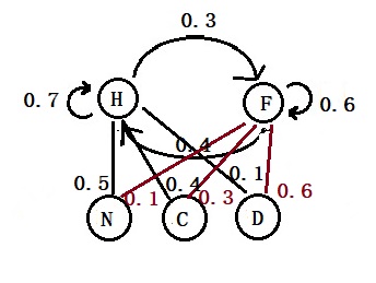
The hidden (latent) variables are “Fever” and “Healthy.” They have translation probabilities.
The observed variables are: “Normal,” “Cold,” and “Dizzy.” They have emission probabilities.

The Viterbi algorithm finds the recursive solution of the most likely state sequence using the maximum a posteriori probability. As the earlier post shows, the Bayes equation may estimate the posterior priority. As the objective is to find the maximum a posteriori, we require only its numerator in Viterbi. In our case,

P(H|N) = P(N|H) x P(H)

H represents “Healthy”, and N denotes “Normal”.

The steps are:
1) Estimate prior probabilities of being healthy (H) or fever (F).
2) Calculate the posterior (the numerator) of day 1 using Bayes.
3) Compare the posteriors of the two posteriors (H vs F) and find out the most likely conditions.
4) Use it as the prior for the next day and repeat steps 2 and 3.

Here is the hidden Markov tree, and we will see the calculations next.
Viterbi algorithm Read More »

Hidden Markov Model – Return of Bayes!

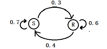
Having seen people’s behaviour—whether wearing a raincoat or not—here is the question: Given that you have seen someone wearing a normal coat, what is the probability that it will be a sunny day? For reference, here is the hidden Markov tree.

In the usual math shorthand, we need to find P(S|NC). We can use the Bayes theorem here.
P(S|NC) = P(NC|S) x P(S) /[P(NC|S) x P(S) + P(NC|R) x P(R)]

P(NC|S) = probability of wearing a normal coat given it’s sunny. We know it is 0.9
P(NC|R) = probability of wearing a normal coat given it’s rainy. It is 0.4
P(S) = prior probability of today being sunny, i.e., without any clues from the dressing.
P(R) = 1 – P(S)

The probability of today being sunny

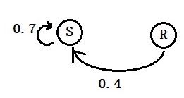
That can be estimated from the transition probabilities as follows. Here is the sunny part of the tree.

S = 0.7 S + 0.4 R

On the other hand,

R = 0.6 R + 0.3 S

To solve the equations, we need one more: S + R = 1. They lead to,

P(S) = 4/7 and P(R) = 3/7.

Back to Bayes

P(NC|S) = 0.9
P(NC|R) = 0.4
P(S) = 4/7
P(R) = 3/7
P(S|NC) = 0.9 x (4/7) /[0.9 x (4/7) + 0.4 x (3/7)]
= (3.6/7) / [(3.6/7) + (1.2/7)] = 3.6/4.8 = 0.75

Hidden Markov Model – Return of Bayes! Read More »

Hidden Markov Model

We have seen how states move from one to another and the translation probabilities. It models a sequence in which the probability of the following (n+1) event depends only on the state of the previous (n) event. That is normal, Markov, where we can see the states. Imagine we can’t directly observe the states but only observe some indications. That is hidden Markov.

An often-used example is observing people’s attire and estimating if it’s sunny or rainy.

If it rains today, there is a 60% chance it will rain the next day and a 40% chance it will be sunny.
If it’s sunny today, there is a 70% chance it will be sunny tomorrow, and 30% will be rainy.

But you can’t observe that. All you see is people wearing a raincoat or normal clothes.
If it rains, there is a 60% chance you will see people wearing raincoats and 40% normal clothes.
If it’s sunny, there is a 90% chance you will see people wearing normal clothes and 10% rain clothes.

Hidden Markov Model Read More »

Waiting for Heads – Four Times

What is the average number of tosses required for a coin to give four consecutive heads?

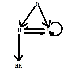
We will solve this as a Markov chain problem. We start with stage 0. At stage 0, two possibilities exist when flipping a coin – H or T. H is counted as one in the right direction, whereas T means you are back to stage 0. From an H, the next flip can lead to HH or 0 with equal probabilities. So, the transition matrix is:

Q <- matrix(c(0.5, 0.5, 0.0, 0.0,
               0.5, 0.0, 0.5, 0.0, 
               0.5, 0.0, 0.0, 0.5, 
               0.5, 0.0, 0.0, 0.0), nrow = 4)

I <- matrix(c(1, 0, 0, 0,
               0, 1, 0, 0, 
               0, 0, 1, 0,
               0, 0, 0, 1), nrow = 4)
I_Q <- I - Q
I_Q_INV <- solve(I_Q)

NN <- c(1, 1, 1, 1)
NN%*%I_Q_INV
30   28   24   16

It takes average 30 moves from 0 to HHHH.

Waiting for Heads – Four Times Read More »

Waiting for Heads – Markov Chains

Some time ago, we analytically estimated the expected waiting times of sequences HT and HH from coin-flipping games. Today, we calculate them using Markov chains.

Waiting time for HT

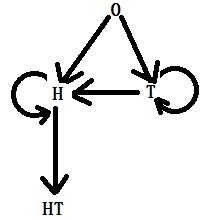
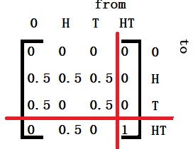
First, the notations, followed by the transition matrix:

\begin{bmatrix} 0.0 & 0.0 & 0.0  & 0.0\\ 0.5 & 0.5 & 0.5  & 0.0\\ 0.5 & 0.0 & 0.5  & 0.0\\ 0.0 & 0.5 & 0.0  & 1.0 \end{bmatrix}

Get Q, I – Q and its inverse 

AA <- matrix(c(0.0, 0.5, 0.5,
               0.0, 0.5, 0.0,
               0.0, 0.5, 0.5), nrow = 3)

II <- matrix(c(1, 0, 0,
               0, 1, 0,
               0, 0, 1), nrow = 3)
BB <- II - AA

CC <- solve(BB)

NN <- c(1, 1, 1)
NN%*%CC
 4    2    4

The average waiting time from 0 to HT is the first element in the vector, i.e., 4.

Waiting time for HH

\begin{bmatrix} 0.0 & 0.0 & 0.0  & 0.0\\ 0.5 & 0.0 & 0.5  & 0.0\\ 0.5 & 0.5 & 0.5  & 0.0\\ 0.0 & 0.5 & 0.0  & 1.0 \end{bmatrix}

AA <- matrix(c(0.0, 0.5, 0.5,
               0.0, 0.0, 0.5,
               0.0, 0.5, 0.5), nrow = 3)

II <- matrix(c(1, 0, 0,
               0, 1, 0,
               0, 0, 1), nrow = 3)
BB <- II - AA

CC <- solve(BB)

NN <- c(1, 1, 1)
NN%*%CC
 6    4    6

The waiting time is 6.

Waiting for Heads – Markov Chains Read More »

Visting Markov Friends – The Eigen Vector Problem

We have seen two ways of solving the end-stage distribution of cities in the example of Amy’s random walk to her friends. Method #1 is to multiply the transition matrix with itself n times and finally multiply with the initial-state distribution. Method #2 is to solve the equation, P X* = X*.

In the matrix form

0.0 0.33  0.0  0.25   0.0
0.5 0.00  0.5  0.25   0.0
0.0 0.33  0.0  0.25   0.0
0.5 0.33  0.5  0.00   1.0
0.0 0.0   0.0  0.25   0.0

There is a third method: find the first eigenvector of the transition matrix and normalise it (i.e., divide it with the sum of elements to make the total distribution 1). We will manage it using an R program that has an inbuilt function to calculate the higher vector.

pM <- matrix(c(0.0, 0.5,  0.0, 0.50, 0.0, 
               0.333, 0.0,  0.333, 0.333, 0.0,
               0.0, 0.5, 0.0, 0.5,  0.0,
               0.25, 0.25,  0.25, 0.0, 0.25,
               0.0, 0.0,  0.0, 1.0, 0.0), nrow = 5)

eigenvec <- eigen(pM)$vectors
first_eigenvec <- eigenvectors[,1]

first_eigenvec/sum(first_eigenvec)
0.16663714 0.25003386 0.16663714 0.33333681 0.08335504

Visting Markov Friends – The Eigen Vector Problem Read More »

Markovian Mouse and Absorbing Chains

Remember the cat-and-mouse game? We calculated the expected time for the mouse on door # 4 to reach the cat. As we know the Markovian technique, we will solve the problem using absorbing chains. Here is the situation with arrows representing the mouse’s stage-by-stage movement.

We follow the steps described in the previous post.
Step 1: Construct the transition probability matrix
Step 2: Isolate I and make Q
Step 3: Subtract Q from the Identity matrix
Step 4: Calculate the inverse of (I – Q)

In step 1, we re-arrange the columns and get the identity matrix cornered.

Q matrix is

And the rest of the calculations,

AA <- matrix(c(0, 0.5, 0, 0, 0,
               0.5, 0, 0.5, 0, 0,
               0, 0.5, 0, 0.5, 0,
               0, 0, 0.5, 0, 0.5,
               0, 0, 0, 0.5, 0), nrow = 5)

II <- matrix(c(1, 0, 0, 0, 0,
               0, 1, 0, 0, 0,
               0, 0, 1, 0, 0,
               0, 0, 0, 1, 0,
               0, 0, 0, 0, 1), nrow = 5)
BB <- II - AA

CC <- solve(BB)

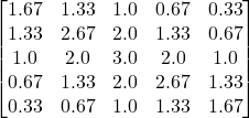
\begin{bmatrix} 1.67  & 1.33 & 1.0  & 0.67 & 0.33\\ 1.33 & 2.67 & 2.0  & 1.33 & 0.67\\ 1.0  & 2.0 & 3.0 & 2.0 & 1.0\\ 0.67 & 1.33 & 2.0  & 2.67 & 1.33\\ 0.33  & 0.67 & 1.0 & 1.33 & 1.67\end{bmatrix}

Add the elements of column 3, which represents door 4. It takes an average of 9 days for the mouse to be caught.

The Cats And Random Mouse Riddle: MindYourDecisions

Markovian Mouse and Absorbing Chains Read More »

Absorbing chains – The Lawfirm

We have seen the concept of absorbing Markov chains. Here is a problem illustrating the idea.

A law firm has three types of employees: junior lawyers, senior lawyers, and partners. During a year
There is a 0.15 probability that a junior will get promoted to a senior
0.05 probability a junior leaves the firm
0.20 probability that a senior will get promoted to a partner
0.1 probability a senior leaves the firm
0.05 probability that a partner leaves the firm

What is the average number of years a junior stays in the company?

Step 1: Construct the transition probability matrix

J stands for junior, S for senior, P for partner, L for leaving and PL for partner leaving

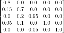
\begin{bmatrix} 0.8  & 0.0 & 0.0  & 0.0 & 0.0\\ 0.15 & 0.7 & 0.0  & 0.0 & 0.0\\ 0.0  & 0.2 & 0.95 & 0.0 & 0.0\\ 0.05 & 0.1 & 0.0  & 1.0 & 0.0\\ 0.0  & 0.0 & 0.05 & 0.0 & 1.0 \end{bmatrix}

Step 2: Isolate I and make Q

If required, re-arrange the transition matrix and identify the unit matrix (corresponding to the absorbing).

After removing the columns and rows corresponding to the identity matrix, you are left with Q.

Q =  \begin{bmatrix} 0.8  & 0.0 & 0.0\\ 0.15 & 0.7 & 0.0\\ 0.0  & 0.2 & 0.95 \end{bmatrix}

Step 3: Subtract Q from the Identity matrix

I - Q =  \begin{bmatrix} 1 & 0 & 0\\ 0 & 1 & 0\\ 0 & 0 & 1 \end{bmatrix} - \begin{bmatrix} 0.8  & 0.0 & 0.0\\ 0.15 & 0.7 & 0.0\\ 0.0  & 0.2 & 0.95 \end{bmatrix}

Step 4: Calculate the inverse of (I – Q)

The whole process so far is

Q <- matrix(c(0.8, 0.15, 0,
               0.0, 0.7, 0.2,
               0, 0.0, 0.95), nrow = 3)

I <- matrix(c(1, 0, 0, 
               0, 1, 0, 
               0, 0, 1), nrow = 3)
I_Q <- I - Q

I_I_Q <- solve(I_Q)
5.0   0.000000    0
2.5   3.333333    0
10.0 13.333333   20

Add numbers corresponding to each category (column) to determine the average number of stages (years). For example, a junior to stay 5 + 2.5 + 10 = 17.5 years. A senior will remain at an average of 3.3 + 13.3 = 16.6, and Partners will persist an average of 20 years before leaving.

Absorbing chains – The Lawfirm Read More »

Markov Chains – Absorbing chains

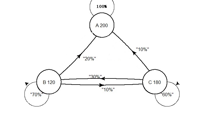
Let’s revisit the three stores. But there is a slight difference this time.

There is no arrow from store A to B or C. The customers who reach A are fully retained or absorbed. This is an absorbing Markov chain. The transition matrix for the above situation is,

\begin{bmatrix} 1 & 0.2 & 0.1\\ 0 & 0.7 & 0.3\\ 0 & 0.1 & 0.6 \end{bmatrix}

You may have guessed it already, but if you continue this chain to develop, the end-state distribution becomes,

\begin{bmatrix} 1 & 0.2 & 0.1\\ 0 & 0.7 & 0.3\\ 0 & 0.1 & 0.6 \end{bmatrix} * \begin{bmatrix} A \\ B \\ C \end{bmatrix} = \begin{bmatrix} A \\ B \\ C \end{bmatrix}

A + 0.2B + 0.1 C = A
0 + 0.7B + 0.3 C = B
0 + 0.1B + 0.6 C = C
A + B + C = 1
A + 1.2B + 1.1 C = 1
0 - 0.3B + 0.3 C = 0
0 + 0.1B - 0.4 C = 0

\begin{bmatrix} A \\ B \\ C \end{bmatrix} = \begin{bmatrix} 1 \\ 0 \\ 0 \end{bmatrix}

Eventually, all customers end up in store A.

Markov Chains – Absorbing chains Read More »

Markov Chains – Visting Friends

Amy lives in city A and has friends in cities B, C, D, and E. The following scheme represents the direct bus connections to these cities. Every Monday, she takes a direct bus at random, reaches the town, and stays with her friend for a week. How many weeks would she have spent in each city that year if she had done this for a year?

The route map suggests that on a given week, Amy has the following probabilities
1) Equal chances from A to B or D (0.5, 0.5)
2) Equal chances from B to A, C, or D (0.33, 0.33, 33)
3) Equal chances from C to B, D (0.5, 0.5)
4) Equal chances from D to A, B, C or E (0.25, 0.25, 0.25, 0.25)
5) Can move from E to D (1.0)

In the matrix form

0.0 0.33  0.0  0.25   0.0
0.5 0.00  0.5  0.25   0.0
0.0 0.33  0.0  0.25   0.0
0.5 0.33  0.5  0.00   1.0
0.0 0.0   0.0  0.25   0.0

The required task is to find the stable end distribution of cities, which can be done using the relationship.

P X* = X*

The expansion of the above equation leads to the following linear relationship that we will solve analytically.

0A + 0.33B + 0C + 0.25D + 0E = A
0.5A + 0B + 0.5C + 0.25D + 0E = B
0A + 0.33B + 0C + 0.25D + 0E = C
0.5A + 0.33B + 0.5C + 0D + 1E = D
0A + 0B + 0C + 0.25D + 0E = E
A + B + C + D + E = 1

Substitute for A in the first equation and solve the set of 5 linear equations using the following R program.

A <- matrix(c( 0.0,   0.5,  0.0,   0.50,  0.0, 
               1.333, -1.0, 0.333, 0.333, 0.0, 
               1.0,   0.5,  -1.0,  0.5,   0.0,  
               1.25,  0.25, 0.25,  -1.0,  0.25, 
               1.0,   0.0,  0.0,   1.0,  -1.0), nrow = 5)
B <- c(1, 0, 0, 0, 0) 

solve(A, B)
0.16686465 0.25007815 0.16661457 0.33335417 0.08333854

Markov Chains – Visting Friends Read More »