March 2024

Placebo, Double-Blind and Experimenter Bias

We have seen the placebo effect. It occurs when someone’s physical or mental condition improves after taking a placebo or ‘fake’ treatment. Placebos are crucial in clinical trials, often serving as effective means to screen out the noise, thereby contributing as the control group to compare the treatment results. Is providing a placebo good enough to remove the biases of a trial?

If the placebo group knows they received the ‘fake pill’, it will nullify its influence. So, the first step in helping the experiment is to hide the information that it is real or placebo from the participants who receive the treatment. This is a single-blind test.

More is needed to prevent what is known as the experimenter bias, also known as the observer expectancy effect. In the next level of refinement, the information is also hidden from the experimenter. This becomes a double-blind experiment. The National Cancer Institute defines it as:
A type of clinical trial in which neither the participants nor the researcher knows which treatment or intervention participants are receiving until the clinical trial is over.”

That means only a third party, who will help with the data analysis, will know the trial details, such as the allocation of groups or the hypothesis. Double-blind studies form the gold standard in evidence-based medical science.

Double-blind study: National Cancer Institute

Placebo, Double-Blind and Experimenter Bias Read More »
Population Distributions vs Sampling Distribution

The purpose of sampling is to determine the behaviour of the population. For the definitions of terms, sample and population, see an earlier post. In a nutshell, population is everything, and a sample is a selected subset.

Population distribution

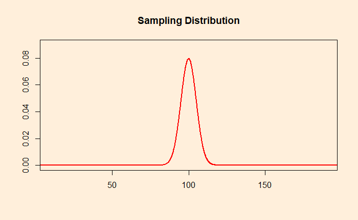
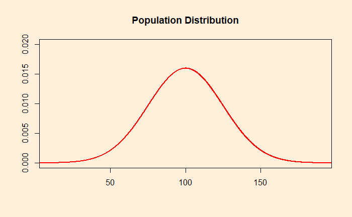
It is a frequency distribution of a feature in the entire population. Imagine a feature (height, weight, rainfall, etc.) of a population with a mean of 100 and a standard deviation of 25; the distribution may look like the following. It is estimated by measuring every individual in the population.

It means many individuals have the feature closer to 100 units and fewer have it at 90 (and 110). Still fewer have 80 (and 120), and very few exceptionals may even have 50 (and 150), etc. Finally, the shape of the curve may not be a perfect bell curve like the above.

Sampling distribution

Here, we take a random sample of size n = 25. Measure the feature of those 25 samples and calculate the mean. It is unlikely to be exactly 100, but something higher or lower. Now, repeat the process for another 25 random samples and compute the mean. Make several such means and plot the histogram. This is the sampling distribution. If the number of means is large enough, the distribution will take a bell curve shape, thanks to the central limit theorem.

In the case of the sampling distribution, the mean is equal to the mean of the original population distribution from which the samples were taken. However, the sampling distribution has a smaller spread. This is because the averages have lower variations than the individual observations.

standard deviation of sampling distribution = standard deviation of population distribution/sqrt(n). The quantity is also called the standard error.

Population Distributions vs Sampling Distribution Read More »

Descriptive statistics and R

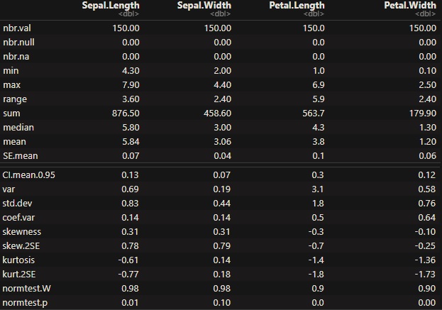
Descriptive statistics summarize various parameters of a dataset. They can be measures of central tendency (e.g., mean, mode, median) or measures of variability (e.g., standard deviation, variance). Here is an R function that describes many of them in one command.

We will use ‘iris’ dataset to illustrate.

dat <- iris
library(pastecs)
stat.desc(dat[1:4], norm = TRUE))

Note that we have rounded off the output to include two digits after the decimal point.

round(stat.desc(dat[1:4], norm = TRUE), 2)

Descriptive statistics and R Read More »

The Central Limit and Hypothesis Testing

The validity of newly explored data from the perspective of the existing population is the foundation of the hypothesis test. The most prominent hypothesis test methods—the Z-test and t-test—use the central limit theorem. The theorem prescribes a normal distribution for key sample statistics, e.g., average, with a spread defined by its standard error. In other words, knowing the population’s mean, standard deviation and the number of observations, one first builds the normal distribution. Here is one example.

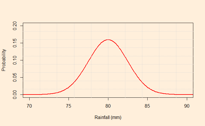
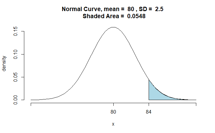
The average rainfall in August for a region is 80 mm, with a standard deviation of 25 mm. What is the probability of observing rainfall in excess of 84 mm this August as an average of 100 samples from the region?

The central limit theorem dictates the distribution to be a normal distribution with mean = 80 and standard deviation = 25/sqrt(100) = 2.5.

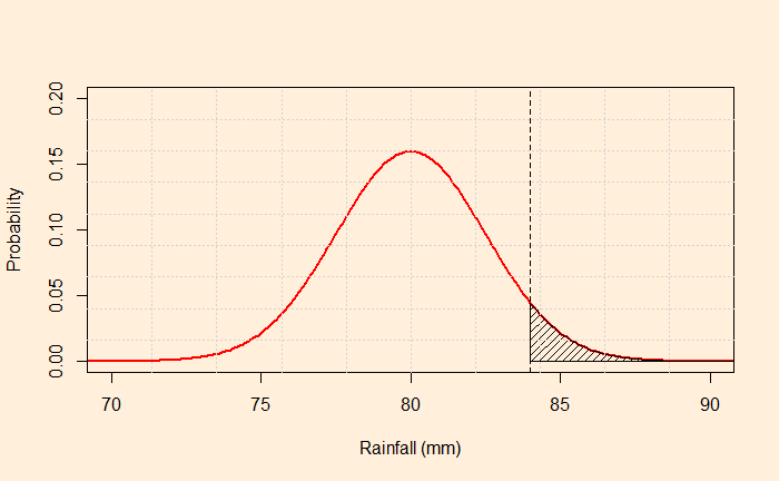
Mark the point corresponds to 84; the required probability is the area under the curve above X = 84 (the shaded region below).

The function, ‘pnormGC’, from the package ‘tigerstats’ can do the job for you in R.

library(tigerstats)
pnormGC(84, region="above", mean=80, sd=2.5,graph=TRUE)

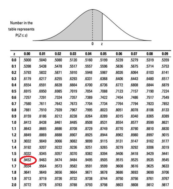
The traditional way is to calculate the Z statistics and determine the probability from the lookup table.

P(Z > [84-80]/2.5) = P(Z > 1.6) 
1 - 0.9452 = 0.0548

Well, you can also use the R command instead of searching in the lookup table.

1 - pnorm(1.6)

The Central Limit and Hypothesis Testing Read More »

Sampling Methods: Non-Probabilistic Sampling

In non-probability sampling, in contrast with its probability analogue, some elements in the population have a zero probability of getting selected or unknown. Because of this, the technique’s representativeness becomes doubtful, and the margin of error becomes uncertain.

Convenience Sampling

As the name suggests, convener sampling picks the samples that are easily accessible. For example, a researcher working on the relationship between coffee drinking and body mass does a survey among her close friends and relatives!

Snowball Sampling

In snowball sampling, initially, a small group of participants are recruited (as per convenience!). The sample is extended by asking the first group to provide their contacts for new participants. And it goes on.

Purposive Sampling

In purposive sampling, the researcher uses her judgment to select the participants. A typical example is seeking expert opinion.

Quota Sampling

It is similar to the strata sampling technique; however, the elements are selected based on convenience sampling.

Sampling Methods: Non-Probabilistic Sampling Read More »

Sampling Methods: Probabilistic Sampling

As we have seen earlier, a statistician estimates the population parameters from the sample parameters. And sampling is the all-important process of selecting subjects or groups that provide the (representative) data required for the work.

Sampling can be of two types – probabilistic and non-probabilistic.

In probabilistic sampling, individual samples are selected based on a known probability distribution. In other words, each element in the group has a known and non-zero probability of being selected. This minimises the risk of systematic bias, i.e., the production of over- or under-representation of sub-groups while picking participants. There are four major types of probabilistic sampling.

Random Sampling

In simple random sampling, each element in the sampling frame has an equal and independent probability of being included. It works well when the population is homogenous. Random sampling is usually done without replacement, although the other possibility – with replacement – is also valid. An easy method is to write down all cases in the population and draw uniform random numbers to select.

Stratified Sampling

In stratified random sampling, the sample is divided into multiple mutually exclusive strata. Sampling then starts from each stratum separately, using random sampling. The separately sampled elements are added together to form the final sample. This technique is critical in less homogenous populations, such that the sample is representative of the strata.

Cluster sampling

In multistage cluster sampling, samples are randomly selected in stages. The steps are:
1) the population is divided into mutually exclusive clusters.
2) use random sampling to select clusters
3) second-level random sampling is done inside the selected clusters to select samples.

Bootstrap aggregating

In bootstrap aggregating or bagging, several samples are generated (or bagged) randomly from the population with replacement. Different analytical methods are developed for each sample.

Sampling Methods: Probabilistic Sampling Read More »

Pascal’s Mugging

Remember Pascal’s Wager? It was an argument for the existence of God based on the idea of a payoff matrix, which is heavily dominated by the case in which God exists. So, the conclusion was to believe in God without seeking evidence. Something similar to Pascal’s wager but doesn’t require infinite rewards is Pascal’s mugging, a concept made by Eliezer Yudkowsky and later elaborated by Nick Bostrom.

Pascal was walking down the street. He was stopped by a shady-looking man asking for his wallet. It was an attempt to mug but without having any arms to threaten the victim. Knowing he has no gun to threaten Pascal, the mugger offers a deal. “Give me your wallet and I will give back double the money tomorrow.”

A utilitarian who trusts the expected value theory can make the following calculations and make a decision:
Imagine I have $10 in my wallet, and the minimum probability expected from the mugger keeping his promise is 50% for a break-even value.
This is because the expected value = – 10 + 0.5 x 20 = 0. Since the shady-looking man is not convincing enough to have such a high chance of repaying, I decide not to hand over my wallet.

Hearing the answer, the mugger increases the deal to 10x. That means if Pascal thinks the mugger has a 1/10 chance of paying 10x, he can hand over the wallet. The answer again was negative. The mugger increases the payment to 1000, 10000, and a million. What would Pascal do?

Now, Pascal is in a dilemma. On the one hand, he knows that the probability that the mugger will pay a million dollars is close to zero, and therefore, he must not hand over the wallet. However, as a rational utilitarian, he can’t ignore the fact that the calculations give a profit if the payback is 1 million dollars.

Pascal’s Mugging Read More »

Winning Russian Roulette

Ana and Becky want to play a safer version of Russian Roulette. The game starts with a coin toss. Whoever wins the toss puts a single round in a six-shot toy revolver, spins the cylinder, places the muzzle against a target, and pulls the trigger. If the loaded chamber aligns with the barrel, the weapon fires, and the player wins.

Given the rules of the game, how important is the toss?

We will evaluate the probability of each player – the one who wins (W) the toss and the one who loses (L).

Let’s write down the scenarios where the toss winner (W) wins the contest.
1) W wins in the first round
2) W doesn’t win in the first, survives the second (L’s chance) and wins the third.
3) W doesn’t win in the first, survives the second (L’s chance), doesn’t win the third, survives the fourth, and wins the fifth.

The total probability of W winning is the sum of all individual probabilities.

1) chance of winning the first round = 1/6
2) chance of winning the third round = chance of not winning the first x chance of not losing the second x chance of winning the third = (5/6)x(5/6)x(1/6) = (1/6)x(5/6)2
3) chance of winning the fifth = (1/6)x(5/6)4
Overall probability = 1/6 + (5/6)x(5/6)x(1/6) = (1/6)x(5/6)2 + (1/6)x(5/6)4 + (1/6)x(5/6)6 + … = 0.545 = 54.5%

On the other hand, the person who lost the toss has a total probability of 45.5% of winning the game. So, a 9% advantage is given by the toss.

Surviving The Deadliest 2-Player Game: Vsauce2

Winning Russian Roulette Read More »

The Carpenter Rule

Here is another problem with conditional probability. There are three men and two women. If one of the men is a carpenter, what is the probability of randomly selecting a carpenter and a man from the group?

Let M represent man, W represents woman, and C represents carpenter.
P(M AND C) = P(M) x P(C|M)
The probability of choosing a man is 3 in 5; the probability that it’s a carpenter, given a man is chosen, is 1/3
= 3/5 x 1/3 = 1/5

This can also be done the following way
P(C AND M) = P(C) x P(M|C)
The probability of choosing a man is 1 in 5; the probability that it’s a man, given it’s a carpenter, is 100%.
= 1/5 x 1 = 1/5

The Carpenter Rule Read More »

Non-Transitive DIce

There are three fair 6-sided dice with the following sides:
A. [2, 2, 4, 4, 9, 9]
B. [1, 1, 6, 6, 8, 8]
C. [3, 3, 5, 5, 7, 7]

If A plays against B, what is the probability of A winning?

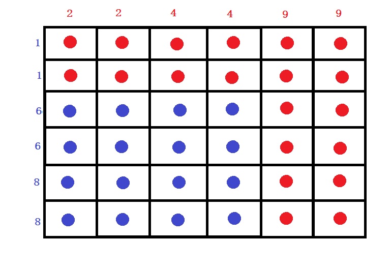
A vs B
The required Probability is:
Probability of rolling a 2 x probability of 2 winning + Probability of rolling a 4 x probability of 4 winning + Probability of rolling a 9 x probability of 9 winning
= (2/6) x (2/6) + (2/6) x (2/6) + (2/6) x 1 = 20/36 = 55.55%

Count the number of red dots and divide it by the total number of dots.

What is the chance of B winning if B plays against C?

B vs C
= (2/6) x (0) + (2/6) x (4/6) + (2/6) x 1 = 20/36 = 55.55%

and

C vs A
= (2/6) x (2/6) + (2/6) x (4/6) + (2/6) x (4/6)= 20/36 = 55.55%

Each die beats the other with a probability of 55.55%.

Non-Transitive DIce Read More »