February 2024

Probability of Circle in a Square

The probability of hitting inside the circle inscribed in a square is a well-known problem. Looking at the geometries, one can find that the required probability is pi/4.

If X is the radius of the circle, then the diameter, 2X, is equivalent to the side of the square. The required probability is the area of the circle (green) over the area of the square. I.e., pi x X2 / (2X) x (2X) = pi / 4. Or four times this probability is pi.

We will do an R code to simulate this case.
Step 1: Create random uniformly distributed points between two equal intervals (-1, 1) to produce a 2 x 2 square.

pts <- 10000
xx <- runif(pts, -1, 1)
yy <- runif(pts, -1, 1)
plot(xx, yy, asp = 1, col = "blue")

Step 2: Select only those points that satisfy the following conditions for a circle: X2 + Y2 < 1, 1 being the circle’s radius that fits inside the square.

for(i in 1:pts){
   if(xx[i]^2 < 1 - yy[i]^2) {
      xx1[i] <- xx[i]
   }else{
      xx1[i] <- 0    
   }
 }
yy1[which(xx1 == 0)] <- 0
plot(xx1, yy1, asp = 1, type = "p", col = "red")

Combining two plots,
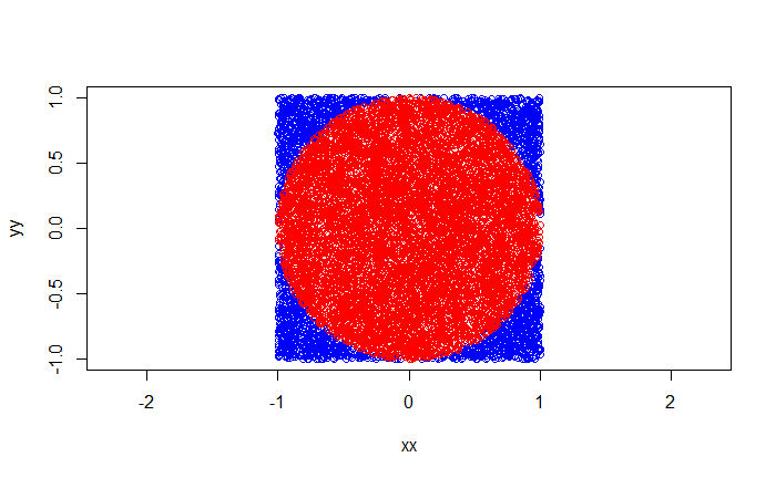
The ratio of the number of points inside the circle to that of the square multiplied by 4 is:

4*length(xx1[abs(xx1) > 0 ]) / length(xx)
3.1456

Tailpiece

Increase the number of points to 100,000, and you get a much cleaner picture:

Probability of Circle in a Square Read More »
Romeo, Juliet and Cofee Meet

Romeo and Juliet plan to meet over coffee between 3 PM and 4 PM. Not known for punctuality, either is willing to wait 15 minutes for the other to show up. What is the probability they will have coffee together?

We will do a graphical solution followed by simulations.

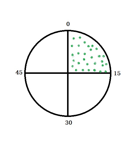
The required probability is the chance of two people meeting inside the shaded area of the circle. It is estimated as 1 – chance of both not making it inside the region = 1 – (3/4)x(3/4) = (16-9)/16 = 7/16 = 0.437.

R Simulations

itr <- 1000000
time_band <- 15

  romeo <- runif(itr, 0, 60)
  juliet <- runif(itr, 0, 60)  
  mean(abs(romeo - juliet) <= time_band)
0.437

Romeo, Juliet and Cofee Meet Read More »

One Crime and Two Suspects

Police know that the crime was committed by one of the two suspects, A and B, with equal evidence against them initially. Further investigation suggests that the blood type of the guilty is found in 1/10 of the population. If A’s blood matches this type, whereas B’s is unknown, what is the probability that A is guilty?

The probability that A is guilty, given his blood matches = P(A|M)
P(A|M) = P(M|A) x P(A) /(P(M|A) x P(A) + P(M|B) x P(B))
P(A|M) = 1 x (1/2) /[1 x (1/2) + (1/10)x (1/2)] = 10/11

One Crime and Two Suspects Read More »

Story Proof for Vandermonde’s identity

Vandermonde’s identity is a famous relationship between binomial coefficients. It has the following form:

_{m+n}C_k = \sum\limits_{j=0}^k _{m}C_j * _{n}C_{k-j}

Blitzstein and Hwang, in their book Introduction to Probability, give a story proof to the identity. Suppose m boys and n girls want to form a committee of k members; there are (m+n)Ck possibilities for doing it. It forms the left-hand side of the identity.

For every j number of boys in the committee, there will be (k-j) girls in it. The number of possibilities is mCj x nCk-j. The required possibility will be the sum of all those possibilities where j ranges from 0 (no boys) to k (only boys).

Story Proof for Vandermonde’s identity Read More »

Bayesian Medicine

A new medicine is developed against a disease to improve the incumbent treatment that is effective in 50% of patients. The expectation is that there is a 2/3 chance that the new treatment will be effective on 60% of patients and a 1/3 chance that the new treatment will be as good as the older one (effective on 50% of patients). The new treatment was given to 20 random patients in the first field trial and was found effective for 15.

With the above information, what is the probability that the new treatment is better than the existing one?

The objective is to find the probability that the new medicine (N) is better, given it was effective on 15 patients in the trial. The notation for this is P(N|X=15) and using Bayes’ theorem,

P(N|X=15) = P(X=15|N) x P(N) / [P(X=15|N) x P(N) + P(X=15|Nc) x P(Nc)]

P(X=15|N) = Probability of getting 15 successes given the probability is 0.6 = 20C15 x (0.6)15 x (0.4)5 (Binomial theorem)
P(X=15|Nc) = Probability of getting 15 successes given the probability is 0.5 = 20C15 x (0.5)15 x (0.5)5 (Binomial theorem)
P(N) = 2/3
P(Nc) = 1/3

dbinom(15, 20, prob = 0.6)*(2/3) / (dbinom(15, 20, prob = 0.6)*(2/3) + dbinom(15, 20, prob = 0.5)*(1/3))
0.91

Bayesian Medicine Read More »

Linear Programming in R – Integer Value Optimisation

In the earlier linear optimization problem, we got the solution as X1 (product 1) = 24 and X2 (product 2) = 16. The interesting thing to notice here is that both are whole numbers; you can’t make and sell fractional products! It may only be the case in some cases. Here is an example.

A factory makes three products: chairs, tables and sofas.
One chair makes $150 profit, requires 7 hours to produce, and 3 m2 of space to store
One table makes $250 profit, requires 9 hours to produce, and 6 m2 of space to store
One sofa makes $300 profit, requires 11 hours to produce, and 7 m2 of space to store

Now, the constraints. The resources available for the factory are only sufficient to cover up to 80 hours a week. The warehouse has an area of 40 m3, and based on historical data, a maximum of 4 chairs sell in a week. Estimate an optimised production plan.

Here is an R code and the results.

f.obj <- c(150, 250, 300)
f.con <- matrix (c(7, 9, 11, 3, 6, 7, 4, 0, 0), nrow = 3, byrow = TRUE)
f.dir <- c("<=", "<=", "<=")
f.rhs <- c(80, 40, 8)
results <- lp ("max", f.obj, f.con, f.dir, f.rhs)
results
results$solution
Success: the objective function is 1757.143 
[1] 2.000000 0.000000 4.857143

While making two chairs a week seems reasonable, it doesn’t make any sense to make 4.85 sofas and expect someone to buy a 0.85 item. At the same time, rounding off to 5 will end up violating the two constraints (on resource and space).
So, we will specify integer constraints to variables 1, 2 and 3 by adding ‘int.vec = ‘ in the options.

f.obj <- c(150, 250, 300)
f.con <- matrix (c(7, 9, 11, 3, 6, 7, 4, 0, 0), nrow = 3, byrow = TRUE)
f.dir <- c("<=", "<=", "<=")
f.rhs <- c(80, 40, 8)
results <- lp ("max", f.obj, f.con, f.dir, f.rhs, int.vec = c(1,2,3))
results
results$solution
Success: the objective function is 1750 
[1] 2 1 4

Reference

Linear Optimization: Desmond C. Ong

Linear Programming in R – Integer Value Optimisation Read More »

Linear Programming in R – Shadow Prices

In the last post, we have seen how R performs linear programming and estimates the limits of the coefficients of the objective function over which the optimal solution remains the same. That was one kind of sensitivity check. The second way is to vary the constraints and observe how the objective function varies. It is the shadow price (of a constraint) and is defined as the change in the objective function value for a unit increase on the right-hand side of the constraint.

To recap, the following is the summary of the objective function and the constraints.

Maximise 45 X1 + 50 X2 (Objective function)
500 X1 + 500 X2 </= 20000 (constraint 1)
750 X1 + 625 X2 </= 42000 (constraint 2)
150 X1 + 100 X2 </= 10400 (constraint 3)
200 X1 + 300 X2 </= 9600 (constraint 4)
X1  </= 50 (constraint 5)
X2  </= 20 (constraint 6)
X1  >/= 0 (constraint 7)
X2  >/= 0 (constraint 8)

Also, recall that the above set of equations gave the maximum profit (the objective function value) of 1880, and the optimal production quantities are alpha = 24 and beta = 16.

The shadow price of constraint 1 is the change in maximum profit from 1880 when the right-hand side of constraint 1 is increased from 20000 to 20001. We can run the code and find out what it is.

f.obj <- c(45, 50)
f.con <- matrix (c(500, 500, 750, 625, 150, 100, 200, 300, 1, 0, 0, 1), nrow = 6, byrow = TRUE)
f.dir <- c("<=", "<=")
f.rhs <- c(20001, 42000, 10400, 9600, 50, 30)

results <- lp ("max", f.obj, f.con, f.dir, f.rhs, compute.sens=TRUE)
results
Success: the objective function is 1880.07 

The value increased by 0.07 (1880.07 – 1880.0). The R can give all the shadow values using the following command. Note that you have added the attribute, ‘compute.sens=TRUE’, in the earlier code.

results$duals
 0.07 0.00 0.00 0.05 0.00 0.00 0.00 0.00

The numbers are the shadow values from constraint 1 to constraint 8. The results show that only a change of one unit of constraint 1 and constraint 4 makes changes in the objective function value. They are, respectively, supply of ingredient A and supply of ingredient D. The former has a shadow value of 0.07, and the latter has 0.05.

Linear Programming in R – Shadow Prices Read More »

Linear Programming in R – What If

In the last post, we did the optimisation of a product line and found that:
The maximum profit is 1880, and the optimal production quantities are alpha = 24 and beta = 16.

Now, a question can arise:
What if we change the objective or the constraints by a little? In other words, how sensitive is the solution to changes in the situation?

One way is to rerun the program with a different coefficient. Let us change alpha’s profit (per kg) from 45 to 47 and see what happens.

library(lpSolve)
f.obj <- c(47, 50)
f.con <- matrix (c(500, 500, 750, 625, 150, 100, 200, 300, 1, 0, 0, 1), nrow = 6, byrow = TRUE)
f.dir <- c("<=", "<=")
f.rhs <- c(20000, 42000, 10400, 9600, 50, 30)

results <- lp ("max", f.obj, f.con, f.dir, f.rhs)
results
results$solution
Success: the objective function is 1928 
24 16

The maximum profit changes to 1928, but the optimal production quantities remain at (24, 16).

What about making it 50? Now, quantities change to (40,0) – produce only alpha!

Rather than making changes manually, the lp function can do it for us using the attribute compute.sens = TRUE . We then use results$sens.coef.from and results1$sens.coef.to to get the range of coefficients.

results <- lp ("max", f.obj, f.con, f.dir, f.rhs, compute.sens=TRUE)
results1$sens.coef.from
results1$sens.coef.to
33.33333 45.00000
50.0 67.5

The solution is optimal as long as the coefficient on X1 stays between [33.33 and 50].
The solution is optimal if the coefficient on X2 is between [45 and 67.5].
Note that you only change one coefficient at a time in sensitivity calculations.

Linear Programming in R – What If Read More »

Linear Programming in R

A factory makes two products, Alpha and Beta, using four ingredients: A, B, C and D. The quantity requirement for each component per kg of the product is:

ABCD
Alpha500750150200
Beta500625100300

The profits from the products (per kg) are

Profit
Alpha45
Beta50

The maximum daily demands for the product (kg) are:

Profit
Alpha50
Beta20

If there are constraints (as below) on the supply of the ingredients, what should be the product mix?

ABCD
2000042000104009600

Linear Programming

This is an example of the application of linear programming (LP), a popular tool in prescriptive analysis. The solution starts by identifying the decision variables and the objective function.

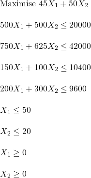
The quantities of the two products are the decision variables. Let’s name them X1 (alpha) and X2 (beta). The objective (function) is to maximise the profit, 45 X1 + 50 X2. All the other information provided above are constraints (on the ingredients, demand, etc). The LP formulation is given below:

\\ \textrm{Maximise } 45 X_1 + 50 X_2 \\ \\ 500 X_1 + 500 X_2 \le 20000 \\ \\ 750 X_1 + 625 X_2 \le 42000 \\ \\ 150 X_1 + 100 X_2 \le 10400 \\ \\ 200 X_1 + 300 X_2 \le 9600 \\ \\ X_1 \le 50 \\ \\ X_2 \le 20 \\ \\ X_1 \ge 0 \\ \\ X_2 \ge 0

We use R to solve the set of equations. The package used is ‘lpSolve’.

library(lpSolve)
f.obj <- c(45, 50)
f.con <- matrix (c(500, 500, 750, 625, 150, 100, 200, 300, 1, 0, 0, 1), nrow = 6, byrow = TRUE)
f.dir <- c("<=", "<=")
f.rhs <- c(20000, 42000, 10400, 9600, 50, 30)

results <- lp ("max", f.obj, f.con, f.dir, f.rhs)
results
results$solution
Success: the objective function is 1880 
24 16

The maximum profit is 1880, and the optimal production quantities are alpha = 24 and beta = 16.

Linear Programming in R Read More »

More Dice Roll

We will consider three instances of utilising the concept of expected values for estimating the number of trials for a given outcome.

Getting a 6

How many times must a 6-sided fair die be rolled for a 6?

There is a 1 in 6 chance that the expected number of rolls is 1, i.e., get a six in the first roll. There is a 5/6 chance that the roll results in another number. In that case, the game will need at least another toss, and the game will repeat. Let E be the expected number of rolls until a 6, using the expected value formula:
E = (1/6)x1 + (5/6) x (E+1)
E = 1 + 5E/6
E = 6

Getting a 66

How many times must a 6-sided fair die be rolled for a 6 followed by a 6?

Let E66 be the required value. We have seen in the earlier section that the expected number of rolls for a six is 6. Once that happens, there is a (1/6) chance that the next roll will give a six and a (5/6) chance that the game will start again.
E66 = 6 + (1/6)x1 + (5/6) x (E66+1)
E66 = 6 + 1 + 5E66/6
E66 = 42

Getting a 65

Here, we estimate the expected number of rolls for a six followed by a number other than six. It is more complicated than the earlier case. After getting the first 6, there are three possibilities:

  1. A 5 and game over.
  2. A 6 and have another chance for a 65 (665).
  3. A number other than 5 or 6 and restart. 

Let E65 be the required value, the expected number of rolls for 65 from the start. We will need to define another term, E6, which is the expected number of rolls for 65 from 6.

E6 = (1/6)x(E6+1) + (4/6)x(E65+1) + (1/6)x1
E65 = (1/6)x(E6+1) + (5/6)x(E65+1)

E65 = 36

More Dice Roll Read More »