June 2023

Pearson vs Spearman Correlations

We have seen Pearson’s correlation coefficient earlier. There is a nonparametric alternative to this which is Spearman’s correlation coefficient.

Pearson’s is a choice when there is continuous data for a pair of variables, and the relationship follows a straight line. Whereas Spearman’s is the choice when you have a pair of continuous variables that do not follow a linear relationship, or you have a couple of ordinal data. Another difference is that Spearman correlates the rank of the variable, unlike Pearson (which uses the variable itself).

Rank of variables

A rank shows the position of the variable if the variable is organised in ascending order. The following is an example of a vector, xx and its rank.

VariableRank
103
21
345
214
52

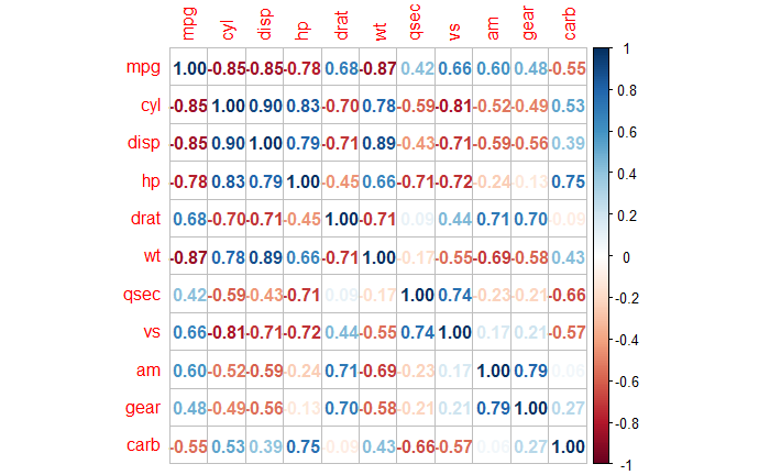
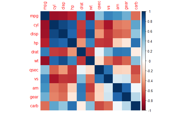
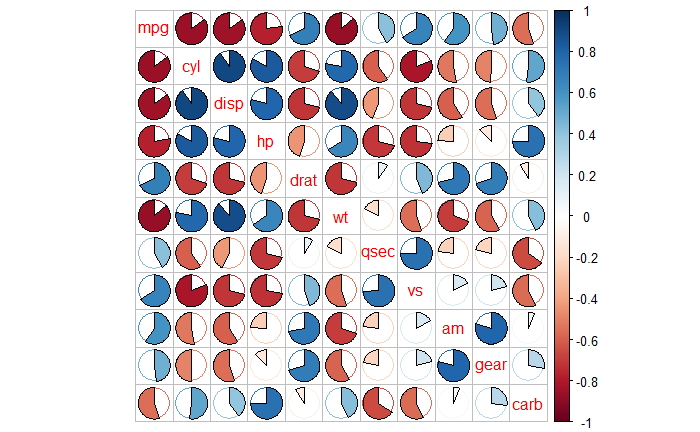
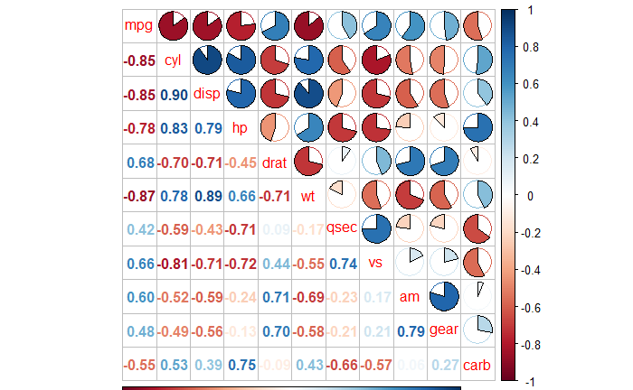
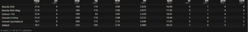
Let’s apply each of the correlation coefficients to the mtcars database.

Pearson Method

cor.test(car_data$mpg, car_data$hp, method = "pearson")
	Pearson's product-moment correlation

data:  car_data$mpg and car_data$hp
t = -6.7424, df = 30, p-value = 1.788e-07
alternative hypothesis: true correlation is not equal to 0
95 percent confidence interval:
 -0.8852686 -0.5860994
sample estimates:
       cor 
-0.7761684 

Spearman Method

cor.test(car_data$mpg, car_data$hp, method = "spearman")
	Spearman's rank correlation rho

data:  car_data$mpg and car_data$hp
S = 10337, p-value = 5.086e-12
alternative hypothesis: true rho is not equal to 0
sample estimates:
       rho 
-0.8946646 

Spearman via Pearson!

cor.test(rank(car_data$mpg), rank(car_data$hp), method = "pearson")
	Pearson's product-moment correlation

data:  rank(car_data$mpg) and rank(car_data$hp)
t = -10.969, df = 30, p-value = 5.086e-12
alternative hypothesis: true correlation is not equal to 0
95 percent confidence interval:
 -0.9477078 -0.7935207
sample estimates:
       cor 
-0.8946646 

Pearson vs Spearman Correlations Read More »

mtcars Dataset – Correlation Plots

In exploratory data analyses, you may want to check the correlations – the strength and the direction – in one go. And a correlation matrix can give that snapshot. Following is the R code to get the matrix.

corrplot(corr = cor(car_data), method = 'number')

As we discussed in the previous posts, a higher positive number (blue) denotes a stronger positive correlation between the variables (pairwise), and the negative (red) indicates the opposite.

Let’s work on various other ways of visualising the same using R.

As a colour map

corrplot(corr = cor(car_data), method = 'color')

As a pie chart and labels inside

corrplot(corr = cor(car_data), method = 'pie', tl.pos = 'd')

Having mixed visualisations for upper and lower triangles

corrplot(cor(car_data), type = 'upper', method = 'pie', tl.pos = "d")
corrplot(cor(car_data), type = 'lower', method = 'number', add = TRUE, tl.pos = "n", diag = FALSE)

mtcars Dataset – Correlation Plots Read More »

mtcars Dataset – Correlation Coefficient

We have seen a couple of plots showing relationships between variables in the ‘mtcars‘ database.

Statisticians use single numbers to quantify the strength and direction of the relationship. One of them is the correlation coefficient which quantifies linear relationships. Before going into correlation coefficients, let’s first learn the covariance between two variables.

Covariance

The sample covariance among two variables based on N observations of each is,

Cov(x,y) = \frac{1}{N-1}\sum\limits^{N}_{i = 1} (x_i - \bar{x}) * (y_i - \bar{y})

You see N − 1 in the denominator rather than N when the population mean is not known and is replaced by the sample mean (X bar).

sum((car_data$mpg - mean(car_data$mpg))*(car_data$cyl - mean(car_data$cyl))) / 31

Or simply,

cov(car_data$mpg, car_data$cyl)
-9.17

Correlation coefficient

The Pearson correlation coefficient is the covariance of the two variables divided by the product of their standard deviations.

r_{x,y} = \frac{Cov(x,y)}{s_xs_y}

cov(car_data$mpg, car_data$cyl) /(sd(car_data$mpg)*sd(car_data$cyl))

Or use the following command from ‘corrplot‘ package

cor(car_data$mpg, car_data$cyl)
-0.85

The greater the absolute value of the correlation coefficient, the stronger the relationship. The maximum value is 1 (+1 and -1), which represents a perfectly linear relationship. A positive value means when one variable increases, the other one also increases. On the other hand, a negative value suggests when one value increases, the other decreases.

In exploratory analyses, however, you may want to know the relationships between several variables in one go. That is the topic for the next post.

References

The Correlation Coefficient: Investopedia
Covariance: Wiki

mtcars Dataset – Correlation Coefficient Read More »

Correlation and mtcars Dataset

‘mtcars’ is a popular dataset which is used to illustrate a bunch of statistical concepts. The data is collected from the 1974 Motor Trend US magazine and comprises fuel consumption and ten aspects of automobile design and performance for 32 automobiles (1973–74 models). It is a built-in dataset in R, and the first few lines may be seen using the following command.

head(mtcars)

The following are the variables in the set.

VariableExplanation
mpgMiles
(US) gallon
cyl# of cylinders
dispDisplacement
(cu.in.)
hpGross horsepower
dratRear axle ratio
wtWeight
(1000 lbs)
qsec1/4 mile time
vsEngine
(0 = V-shaped,
1 = straight)
amTransmission
(0 = automatic,
1 = manual)
gear# of forward gears
carb# of carburettors

The data enables one to find out the relationship between the different characteristics with the fuel efficiency of cars. E.g., the following plot relates the miles per gallon with the number of cylinders.

Or how the gross horsepower is related to the number of cylinders.

Correlation and mtcars Dataset Read More »

Temperature Anomaly – Warming Stripes

We have seen the spiral plot and ridgeline plot visualising the temperature anomaly (compared to the 1961-80 average). Today, we make another fancy plot – Warming Stripes – using R (again, courtesy: Ed Hawkins of the University of Reading). The data used here is the same as that we described in an earlier post.

c_data %>% ggplot(aes(x = Year, y = 1, fill = T_diff)) +
geom_tile()+
scale_y_continuous(expand = c(0, 0)) +
            scale_fill_gradientn(colors = rev(brewer.pal(11, "RdBu")))+
            guides(fill = guide_colorbar(barwidth = 1))+
            labs(title = "",
            caption = "")+
            theme_minimal() +
            theme(axis.text.y = element_blank(),
                       axis.line.y = element_blank(),
                       axis.title = element_blank(),
                       panel.grid.major = element_blank(),
                       legend.title = element_blank(),
                       axis.text.x = element_text(vjust = 3),
                       panel.grid.minor = element_blank(),
                       plot.title = element_text(size = 14, face = "bold"),
                       panel.background = element_rect(fill = "black"), 
                       plot.background = element_rect(fill = "black"),
                       axis.text = element_text(color = "white"),
                       legend.text = element_text(color = "white")
                       )

Temperature Anomaly – Warming Stripes Read More »

IESDS -The Cards Game

Amy and Becky are playing a game. Six cards – numbered 1 through 6 – are placed face down on the table. The cards are shuffled, and each one takes a card at random. The person with the higher number wins. Amy looks at her card and finds it is #2. Becky looks at hers and asks if Amy wants to trade her card. What should Amy’s response be? Note both players are rational.

If Becky had a 6, she wouldn’t ask for a trade, as #6 is guaranteed to win. If she had #5, the only card she benefits from is #6, something Amy would never trade. That eliminates #5 and #6 from the game. By extending the logic, 4 and 3 are also eliminated. That leaves #1 something Becky is happy to offer, but Amy will never accept.

So Amy’s answer to the call is a NO.

These types of games are known as the Iterated Elimination of Strictly Dominated Strategies (IESDS).

IESDS -The Cards Game Read More »

Temperature Anomaly – The Ridgeline plot

We have seen the temperature anomaly distribution visualised through a spiral plot. This time it’s another cool one – the ridge plot.

library(tidyverse)
library(ggridges)

c1_data <- c_data %>% group_by(Year) %>% mutate(T_av = mean(T_diff))

c1_data %>% filter(Year > 1950 & Year < 2022) %>% 
  ggplot(aes(x = T_diff, y = factor(Year, levels = seq(2021, 1950, -1)), fill = T_av )) +
  geom_density_ridges(bandwidth = 0.1, scale = 4, size = 0.1, color = "white") +
  scale_fill_gradient2(low = "darkblue", mid = "white", high = "darkred", midpoint = 0, guide = "none") +
  coord_cartesian(xlim = c(-1, 3)) +  
  scale_x_continuous(breaks = seq(-1, 2, 0.5)) +
  scale_y_discrete(breaks = seq(1950, 2020, 10)) + 
  labs(y = NULL, x = "Temperature Anomaly (\u00B0C)", title = "Temperature Anomaly Distribution") +
  theme(text = element_text(color = "white"), 
        panel.background = element_rect(fill = "black"), 
        plot.background = element_rect(fill = "black"),
        panel.grid = element_blank(),
        axis.text = element_text(color = "white"),
        axis.ticks = element_line(color = "white")) 

For the data and clean-up, see the earlier post.

Ridgeline plot in R with ggridges: Riffomonas Project

Temperature Anomaly – The Ridgeline plot Read More »

The Climate Spiral – The Spiral with Plotly

In the last post, we initiated the plotting of the abnormal temperature differences over the years (from the standardised values) thought to have been arising out of global warming. Today, we will build the famous spiral plot to visualise it.

First, we transform the data to polar coordinates.

c_data <- c_data %>% select(Year, all_of(month.abb)) %>% 
  pivot_longer(-Year, names_to = "Month", values_to = "T_diff") %>%
  mutate(Month = factor(Month, levels = month.abb)) %>%
  mutate(Month_no = as.numeric(Month), radius = T_diff + 1.5, theta = 2*pi*(Month_no-1)/12, x = radius * sin(theta), y = radius * cos(theta), z = Year)

The input (the original table) and the output (the transformed table) are presented below.

Plotly

Plotly is an open-source graphing library, which also has one for R (plotly).

plot_ly(c_data, x = ~x, y = ~y, z = ~z, type = 'scatter3d', mode = 'lines',
        opacity = 1, line = list(width = 6, color = ~T_diff, reverscale = FALSE))

The Climate Spiral – The Spiral with Plotly Read More »

The Climate Spiral

Let’s construct a visualisation of global temperature change – from 1880 – similar to what the British climate scientist Ed Hawkins did. The data used in the exercise has been downloaded from the GitHub channel of Riffomonas. He tabulated the deviation in the annual global mean from the data normalized between the temperatures 1951 – 1980.

The first step is to pivot the data into the following format:

c_data <- read.csv("./climate.csv")

c_data <- c_data %>% select(Year, all_of(month.abb)) %>% 
  pivot_longer(-Year, names_to = "Month", values_to = "T_diff") %>%
  mutate(Month = factor(Month, levels = month.abb)) %>%
  mutate(Month_no = as.numeric(Month))

Next, we plot the data we built.

c_data %>% ggplot(aes(x = Month_no, y = T_diff, group = Year, color = Year)) +
  geom_line() + 
  scale_x_continuous(breaks = 1:12, labels = month.abb) +
  scale_y_continuous(breaks = seq(-2, 2, 0.2)) +
  coord_cartesian()

Add a line to change to polar coordinates.

c_data %>% ggplot(aes(x = Month_no, y = T_diff, group = Year, color = Year)) +
  geom_line() + 
  scale_x_continuous(breaks = 1:12, labels = month.abb) +
  scale_y_continuous(breaks = seq(-2, 2, 0.2)) +
  coord_polar()

Climate data: Riffomonas

Riffomonas Project: Youtube

Climate spiral: Wiki

The Climate Spiral Read More »

Probability of Condom Failure

As per CDC, male condoms as a contraceptive has a failure rate of 13% for typical use and 3% for perfect use. The question is: what does it mean? The website doesn’t clarify further.

Possibility 1: a woman will get 13% of the times she has sex using a condom.

If that is true, using the protection once a month (during fertile days), a binomial equation tells you there is an 81% chance of getting pregnant in a year; (1 – (1-0.13)12)*100 = 81. It is no different from the approximate chances of conception for a woman without fertility issues.

The correct interpretation of the statistic is that it’s the number of pregnancies when 100 women use that birth control method for one year. Putting the number 0.13 back in the binomial equation, one can get the condom failure probability of about a per cent. That is pretty impressive.

1 – (0.988)12 = 0.13

References

Contraception: CDC
Statistically safe sex: Math Careers
Interpreting Birth Control Failure Rates: Very well health
Chances of getting pregnant: Medical news today
Risk Savvy: Gerd Gigerenzer

Probability of Condom Failure Read More »