May 2023

Betting on Craps

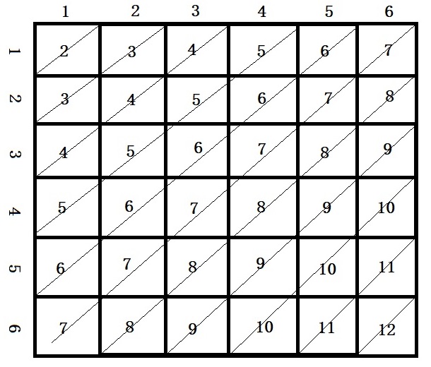
Craps is another popular casino game that involves throwing two dice and noting the total. A person can place several bets, and we discuss the probabilities of one such type – the pass bets. But before we get to the rules, look at how the totals distribute.

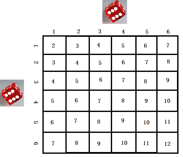
From the picture, you can estimate the probability of each sum as the ratio between the number of occurrences of that number with the total number, i.e., 36. The following picture can help count those possibilities to build the table below.

Dice
Roll
Probability%
21/362.78
32/365.56
43/368.33
54/3611.11
65/3613.89
76/3616.67
85/3613.89
94/3611.11
103/368.33
112/365.56
121/362.78

Pass line bet

The rules for the pass-line bet are:
1) The player throws the dice and wins at once if the total for the first throw is 7 or 11.
2) The player loses if the outcome is 2, 3 or 12.
3) The throws 4, 5, 6, 8, 9 or 10 is called a point.
4) If the first throw is a point, it is repeated until the same number (the point) comes back (player wins) or 7 (player loses).

Now, what are the chances for the player to win a pass-line bet? That is next.

Betting on Craps Read More »

The trouble with Multiple Testing

Last time we saw the issue with sub-group analysis, an example of multiple-hypothesis testing. Here, we illustrate the problem with multiple hypothesis testing. Before that, a few recaps.

  1. Hypothesis testing is a statistical procedure to put assumptions (hypotheses) about a population parameter to test based on evidence collected from samples.
  2. The Null hypothesis is the default assumption (what we assume is true before evidence)
  3. Alpha (significance level) represents the strength of the evidence that must be present in your sample that the effect is statistically significant
  4. p-value is the probability that the observed statistics appeared purely by chance.
  5. if p < alpha, the null hypothesis is rejected
  6. A type I error is when the Null hypothesis is true but you rejected it.
  7. Rejection of the null hypothesis may be called a discovery

Based on item # 6, the probability of type I error is alpha.

Assume five tests are done at a 5% significance level, and the null hypothesis is true. What is the probability that at least one of the tests rejects the null hypothesis?

We know the old formula: at least one = 1 – none. Therefore, at least one type I error = 1 – no type I error = 1 – (1-alpha)5.

1 – (1- 0.05)5 = 0.226 or 22.6%

So, we have a 22.6% chance of rejecting at least one null hypothesis (and making a type I error).

The trouble with Multiple Testing Read More »

False Discovery Rate

I recommend you read the recent post on p-value first. In short, if the investigator rejects the null hypothesis based on evidence, it may be called a discovery. Then what is a false discovery rate (FDR)?

FDR is the proportion of tests in which the null hypothesis is true out of all cases where it is rejected. In probability notation, FDR = P(H0 is true | reject H0).

At first glance, it may resemble the significance level or alpha. But alpha is the probability of rejecting the null hypothesis when it is true; it is P(reject H0 | H0 is true). So, to get the FDR, we need to use Bayes’ theorem.

FDR = P(H0 is true | reject H0) = P(reject H0 | H0 is true) x P(H0 is true) /(P(reject H0 | H0 is true) x P(H0 is true) + P(reject H0 | H0 is not true) x P(H0 is not true))

P(H_0 True | Reject H_0) = \frac{P(Reject H_0 | H_0  True) * P(H_0 True)} {P(Reject H_0 | H_0 True) * P(H_0 True) + P(Reject H_0 | H_0 Not True) * P(H_0 Not True)}

The first term, P(reject H0 | H0 is true), as we know, is alpha. The next one, P(H0 is true), is the prior probability for the null hypothesis to be true that we need to find out. P(H0 is not true) = 1 – P(H0 is true). That leaves the last term, P(reject H0 | H0 is not true). We know the chance of not rejecting if H0 is not true is beta (false-negative or type II error). So, P(reject H0 | H0 is not true) = 1 – beta.

Let’s assume alpha = 0.05, the prior probability of the null hypothesis is 0.25, beta = 0.2,

FDR = \frac{0.05 * 0.25}{0.05 * 0.25 + (1-0.2)*(1-0.25)} = 0.02

False Discovery Rate Read More »

Troubles with Sub-Group Analysis

Here is an example from Dr Vickers’s book, ‘What is a p-value anyway?’ about issues related to investigators running more analyses hoping to get statistical significance. A well-known type is a sub-group analysis. Note the following data on cancer drugs.

New.DrugOld.Drug
Recurred150190
Cancer free850810

Run a Fisher’s Exact Test, and you get a p-value of 0.02, which is statistically significant that the new drug is more effective.

p-value = 0.02016
alternative hypothesis: true odds ratio is not equal to 1
95 percent confidence interval:
 0.5904410 0.9576516
sample estimates:
odds ratio 
  0.752434

Now, you do two sub-groups:

MENNew.DrugOld.Drug
Recurred80100
Cancer free420400
WOMENNew.DrugOld.Drug
Recurred7090
Cancer free430410

Run the test for the first sub-group (men): p-value = 0.12, and for the second (women), the p-value = 0.1; the new drug work for people, but not for men or for women!

Reference

What is a p-value anyway? 34 Stories to Help You Actually Understand Statistics:  Andrew Vickers

Troubles with Sub-Group Analysis Read More »

Hooping with Jordan

Dr Andrew J. Vickers’ famous ‘Hoop story with Jordan’ describes a good interpretation of p-value and hypothesis testing. The story goes like this:

The other day I shot baskets with Michael Jordan. He shot 7 straight free throws; I hit 3 and missed 4 and then rushed to the sideline, grabbed my laptop and calculated a p-value by Fisher’s exact test.

Andrew Vickers, What is a p-value anyway? 34 Stories to Help You Actually Understand Statistics 

So, what was the p-value? Let’s summarise the results and apply the test using R codes.

BasketNo.Basket
Jordan70
Vickers34
hoop.game
hoop.game <- data.frame("Basket" = c(7, 3), "No Basket" = c(0, 4), row.names = c("Jordan", "Vickers"))
fisher.test(hoop.game)
Fisher's Exact Test for Count Data

data:  hoop.game
p-value = 0.06993
alternative hypothesis: true odds ratio is not equal to 1
95 percent confidence interval:
 0.8498871       Inf
sample estimates:
odds ratio 
       Inf 

Now, would you take this p-value (0.07) to suggest that there is no difference between my basketball skills and those of Michael Jordan? The answer is a firm NO; it only says the experiment hadn’t proved a difference between the two players.

Reference

What is a p-value anyway? 34 Stories to Help You Actually Understand Statistics:  Andrew Vickers

Low-Fat Diets Flub a Test: NYT

Hooping with Jordan Read More »

p-value Revisited

Hypothesis testing is an all-important tool in experimental research, needless to say, in pharmaceutical studies and drug discovery. If you forgot, hypothesis testing is a method that determines the probability that an event occurs only by chance.

The word used here is ‘hypothesis’, which suggests some default position (‘no effect’ or Null Hypothesis), and the trial aspires to examine whether the intervention (e.g. consumption of medicine) has made a difference. In other words, if the experimental results reject the null hypothesis, a discovery has happened.

Then you have the popular p-value approach that quantifies and helps the decision-making to reject or not. The experimenter sets a significance level before looking at the p-value. The significance level gives protection against incorrectly making a discovery – it is the probability of rejecting the default when it is true (a.k.a. Type I Error)! The smaller the value, the stronger the required evidence be. A simple coin-flipping example shows you how tough discovery (rejection of null hypothesis) is. I have flipped a coin ten times and got eight heads. Do I have sufficient evidence to prove that the coin is biased toward the heads?

Let’s assume a commonly used significance level of 0.05 (5%). My null hypothesis, naturally, is that the coin is fair (unbiased, with an equal probability of leaning heads or tails). We will use the binomial equation to estimate the chance of getting eight or more heads for an unbiased coin.

P(H >/= 8) = P(H = 8) + P(H = 9) + P(H = 10) = 10C8 x (0.5)8 x (0.5)2 +  10C9 x (0.5)9 x (0.5)1 +  10C10 x (0.5)10 x (0.5)0 = 0.044 + 0.0098 +  0.00098 = 0.055

The following R code can do it in one line.

binom.test(8, 10, 0.5, alternative="greater") 
Exact binomial test

data:  8 and 10
number of successes = 8, number of trials = 10, p-value = 0.05469
alternative hypothesis: true probability of success is greater than 0.5
95 percent confidence interval:
 0.4930987 1.0000000
sample estimates:
probability of success 
                   0.8 

p > the significance value. So, even eight heads out of ten tries can’t prove the coin is biased towards heads. Imagine you wanted to be doubly strict about the trial and set a tighter significance value of 1%, then even 9 out of 10 would have failed the test (p-value = 0.01074 > 0.01)!

Now, you can imagine why the ‘Valley of Death’ exists in clinical research.
p-value Revisited Read More »

McKinsey Curve – Energy Efficiency

If you have noticed the McKinsey curve, and I’m sure you have, one thing that surprises me is why a significant portion of the graph has abatement cost in negative, yet haven’t happened yet! Simple economics can’t explain that. So why does it remain a resource untapped?

One possible explanation can be a lack of information.

Second, is a principal-agent problem

Reference

McKinsey Curve

McKinsey Curve – Energy Efficiency Read More »

McKinsey Curve

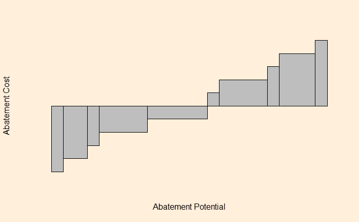
McKinsey curve is a global mapping of opportunities that can reduce GHG emissions and is quite influential among policymakers. These are GHG abatement curves estimated at a future period for different countries. Following is an illustration of how they appear (for getting the actual curves, follow the link in the reference).

For an economist, it is a supply curve or the map of the marginal cost of making the marginal unit. Or the cost of reducing that last ton of greenhouse gas emissions. And each block represents one item – residential lighting, cellulosic biofuel, onshore wind, and coal power plant with CCS, to name a few.

Take one block, say the residential lighting: its width represents how many fewer greenhouse gas emissions we would have if we optimize the residential lighting system. The height is how much would that cost ($/ton CO2) to the households. If it is negative, it suggests the family gains money.

Most items on the negative side (the left side) are related to energy efficiency. And, by the definition of efficient markets, should happen by default, like changing CFL lamps with LED. But it’s a different matter altogether that these don’t always happen that way. But what is the idea of getting everything done on the list? From an economist’s standpoint, add a carbon tax larger than the height of the highest block on the right side. It becomes cheaper to perform abatement in that sector than pay taxes.

Reference

McKinsey Curve

McKinsey Curve Read More »

The Misuse of Conditional Probabilities

The misuse of conditional probability was at its best (worst) in the OJ Simpson murder trial. To give a one-line summary of the context, in June 1994, the American footballer O J Simpson was arrested and charged with the murders of his ex-wife Brown and her friend Goldman.

Against the prosecutor’s argument that Mr Simpson had a history of violence towards his wife, the defence argued that 1 in 2500 of the men who abuse their wives end up murdering them. And the judge seemed to have bought this conditional probability that

P(Husband murders wife | Husband abuses wife) = 1/2500

The real conditional probability should have been

P(Abusive husband is guilty | The wife is murdered)

The probability for this is much higher, close to 80%.

The Misuse of Conditional Probabilities Read More »

The Elevator Paradox

The elevator problem is an observation reported by physicists Marvin Stern and George Gamow. They observed that someone who waits for an elevator (to go down) at one of the top floors (not the topmost) is more likely to see the first elevator that stops at the floor going up.

Imagine the building has 20 floors, and the person who wants to go down has her office on the 19th. The elevator is in constant flight, and it takes 1 second to cover one floor. Let’s write down a hypothetical journey.

FloorUpDown
205:00:38
195:00:374:59:59; 5:00:39
18365:00; 40
173501
163402
153303
143204
133105
123006
112907
102808
92709
82610
72511
62412
52313
42214
32115
22016
11917
05:00:1818

Everyone who comes between 5:00 and 5:00:37 sees the elevator going up (at 5:00:37) and only the people who reached floor 19 at 5:00:38 and 5:00:39 miss that (and only see it comes down from floor 20).

The Elevator Paradox Read More »