May 2023

Collider Bias – The Math

So far, I have addressed the collider-bias phenomena qualitatively. This time, I will try to show through numbers. It can be complex as the illustration involves a lot of arithmetic. The reference material provided at the end is a good read, further grasping the concept.

Imagine a situation where exposure is obesity, the risk factor is smoking, the outcome is mortality, and the collider is diabetes. If you are confused about what each represents, here is the expected storyline: A research group does study the impact of obesity on mortality in a set of people who have diabetes and comes up with a counterintuitive conclusion (perhaps that obesity decreases mortality)!

Set of information

Total study population = 1000
Smokers = 500
Non-smokers = 500
Obese = 500
Non-obese = 500
Baseline diabetes risk (non-smoking, non-obese)= 4%
Obesity increases diabetes risk by 16 % points
Smoking increases diabetes risk by 12% points
Baseline mortality risk (non-smoking, non-obese, nondiabetic)= 5%
Obesity increases mortality risk by 2.5% points
Smoking increases mortality risk by 15% points
Diabetic increases mortality by 5%

Calculations on the total sample

The overall study population is depicted as

Now, calculate the mortality rates of each quadrant and portion into obesity and non-obesity conditions.

Total mortality of NS-NO (non-smoking, non-obese) quadrant
= # of diabetic x diabetic mortality + # non-diabetic x baseline mortality
= 0.04 x 250 x (0.05 + 0.05) + (250 – 0.04 x 250) x 0.05
= 1 + 12 = 13
(note that diabetic mortality = baseline mortality + diabetic increases mortality)

S-NO (smoking, non-obese) quadrant
= # of diabetic x (diabetic mortality + smoking mortality) + # non-diabetic x (Baseline mortality + smoking mortality)
= (0.04 + 0.12) x 250 x (0.05 + 0.05 + 0.15) + (250 – (0.04 + 0.12) x 250) x (0.05 + 0.15)
= 52

S-O (smoking, obese) quadrant
= (0.04 + 0.12 + 0.16) x 250 x (0.05 + 0.05 + 0.15 + 0.025) + (250 – (0.04 + 0.12 + 0.16) x 250) x (0.05 + 0.15 + 0.025)
= 60

NS-O (non-smoking, obese) quadrant
= (0.04 + 0.16) x 250 x (0.05 + 0.05 + 0.025) + (250 – (0.04 + 0.16) x 250) x (0.05 + 0.025)
= 21
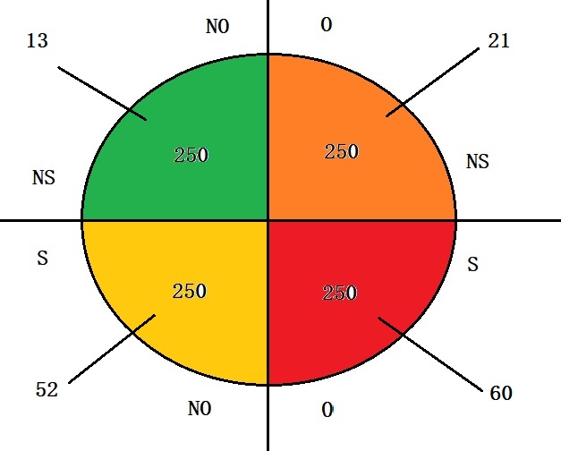
Calculations (for the total sample)
Mortality rate with obesity = (60 + 21) / 500 = 16.5%
Mortality rate without obesity = (13 + 52) / 500 = 13%
An increase of 3.5%

Calculations on the sub-sample

Suppose the study stratified the sample and analysed only people who have diabetes. The study sample space is as follows.

Do the same exercise as before

NS-NO quadrant
= # of diabetic x diabetic mortality
= 0.04 x 250 x (0.05 + 0.05)
= 1

S-NO quadrant
= # of diabetic x (diabetic mortality + smoking mortality)
= (0.04 + 0.12) x 250 x (0.05 + 0.05 + 0.15)
= 10

S-O quadrant
= (0.04 + 0.12 + 0.16) x 250 x (0.05 + 0.05 + 0.15 + 0.025)
= 22

NS-O quadrant
= (0.04 + 0.16) x 250 x (0.05 + 0.05 + 0.025)
= 6
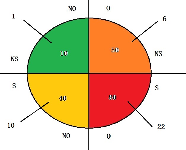
Calculations (for the sub-sample)
Mortality rate with obesity = (22 + 6) / 130= 21.5%
Mortality rate without obesity = (1 + 10) / 50= 22 %
A decrease of 0.5%

Reference

Collider Bias in Observational Studies: Dtsch Arztebl Int.

Collider Bias – The Math Read More »

The Obesity Paradox

The obesity paradox is the idea that people who are overweight live longer than normal-weight people. While later studies have found this claim invalid, the notion stayed in public discourse ever since.

There are many explanations for this odd observation. One of them goes with the parameter of measurement itself – the survival rate after getting cardiovascular disease. Studies found that obese people may get the disease much earlier in life and therefore survive a longer proportion of life with it.

Another one is collider stratification bias, which happens when two variables, e.g., risk factor and outcome, influence a third, namely, the likelihood of being sampled. It works in the following way:

Obese individuals may have developed CAD because they are obese or because of another stronger condition, e.g., smoking or genetics. In other words, CAD, the collider, is caused by 1) obesity and 2) the (more severe) condition (smoking). In this simple two-cause model, a stratification of variables means among individuals with CAD, obese individuals are less likely to be smokers, and non-obese individuals are more likely to be smokers. Subsequently, obesity may appear protective against mortality (outcome) because its presence indicates the absence of a more harmful risk factor – smoking.

References

The ‘obesity paradox’ may not be a paradox at all: International Journal of Obesity

Obesity is bad regardless of the obesity paradox for hypertension and heart disease: J Clin Hypertens

Association of Body Mass Index With Lifetime Risk of Cardiovascular Disease and Compression of Morbidity: JAMA Cardiology

The Obesity Paradox Read More »

Night Light and Myopia

A well-known case for confounding was the finding of night lighting casing myopia in young children.

In 1999 Quinn et al. published an article in the prestigious journal Nature that reported a strong association between exposure to nighttime light before the age of two years and myopia and created wide publicity in the media. As axial myopia is caused by excessive eyeball growth during childhood, the researchers rationalised that nighttime lighting in young children could stimulate the condition.

However, multiple studies that repeated the investigation found no association between the exposure (night light) and the outcome (myopia).

Myopic parents

It turned out that the fault was from those myopic parents of those infants who had the habit of keeping the lights on at night for better vision and created the confounder. As myopic parents tend to have myopic children, the association now looked easier to understand.

References

Myopia and ambient lighting at night: Quinn et al.
Continuous ambient lighting and eye growth in primates: Smith et al.
Myopia and night lighting in children in Singapore: Saw et al.

Night Light and Myopia Read More »

Criteria for Confounders

Identifying confounders is a challenge that statisticians encounter all the time. Confounding determines whether or not a causal association exists between an exposure and an outcome. A (rather silly) example is the notion that carrying matchboxes causes lung cancer. The factor – confounder – here is the smoking status. Smokers are likely to carry matchboxes; smokers have a higher chance of getting lung cancer. If this confounder is not identified, one may conclude that having matchboxes is the exposure that caused the outcome of lung cancer.

As per Jager et al., a confounding variable must satisfy three criteria: 1) it must have an association with the exposure of interest, (2) it must be associated with the outcome of interest, and (3) it must not be an outcome of the exposure.

Criteria for Confounders Read More »

Physical Activity and Health

The March issue of the British Journal of Sports Medicine came out with the results from a 9-year-long cohort study of people who did physical activity and its impact on influenza and pneumonia.

Before we get into details, note that it is a cohort study – of 577 909 US adults. Cohort studies are observational, whereas randomised controlled trials (RCTs) are interventional. Establishing causations from observational studies is problematic.

A key finding of the study has been the association of lowered risk of influenza and pneumonia with aerobic physical activity.

Reference

Webber BJ, et al. Br J Sports Med 2023;0:1–8.

Physical Activity and Health Read More »

Fisher’s Exact Test

Fisher’s exact test is a statistical significance test that calculates the p-value and indicates an association between two variables. For example, scientists tagged 50 king penguins in each of three nesting areas (lower, middle, and upper) and counted the numbers that were alive or dead after a year. The following were the results.

AliveDead
Upper nesting area437
Middle nesting area446
Lower nesting area491

Are these differences significant?

penguin.nest <- data.frame("Alive" = c(43, 44, 49), "Dead" = c(7, 6, 1), row.names = c("Lower", "Middle", "Upper"))
fisher.test(penguin.nest)

The p-value is 0.0896; it is not significant.

Fisher’s Exact Test Read More »

Hypergeometry of counterfeits

A collection of 15 gold coins contains 4 counterfeits. If 2 of them are randomly selected to be sold at the auction, find the probability that

  1. neither of them is a counterfeit
  2. only one of them is a counterfeit
  3. both coins are counterfeits.

This is a hypergeometric probability distribution – picking without replacement. If X is the number of counterfeit coins (hypergeometric random variable),

P(X = 0) = \frac{_{4}C_0 \textrm{ }*\textrm{ } _{11}C_2\textrm{ }}{_{15}C_2}

choose(4,0)*choose(11,2) / choose(15,2)
0.52

P(X = 1) = \frac{_{4}C_1 \textrm{ }*\textrm{ } _{11}C_1\textrm{ }}{_{15}C_2}

choose(4,1)*choose(11,1) / choose(15,2)
0.42

P(X = 2) = \frac{_{4}C_2 \textrm{ }*\textrm{ } _{11}C_0\textrm{ }}{_{15}C_2}

choose(4,2)*choose(11,0) / choose(15,2)
0.06

Or simply,

dhyper(2, 4, 11, 2, log = FALSE)

Hypergeometry of counterfeits Read More »

Coffee Overflow

A coffee machine is regulated to charge 195 ml per cup with a standard deviation of 5 ml. Assuming the amount of fill is normally distributed, what is the probability that 200 ml cups will overflow?

For normal distributions,

P(X \ge 200) = P(z \ge \frac{200-\mu}{\sigma})  = P(z \ge \frac{200-195}{5})

Or you may use this simple R command

1 - pnorm(200, 195, 5)
0.1586553

Coffee Overflow Read More »

Craps Probability – Don’t Pass

Another type of bet in craps is a ‘don’t pass bet’. Here, the winning opportunities are the opposite of what we have seen before. Well, not really; had that been the case, the player would have got an exactly opposite, +1.41% advantage, which is absurd. A player never holds winning odds in gambling! The rules are almost the opposite, but getting 12 in the first throw makes a pass (no win. no loss). Let’s list down all the possible outcomes and the payoff table.

  1. The player throws the dice and wins at once if the total for the first throw is 2 or 3.
  2. The player loses if the outcome is 7 or 11.
  3. It’s a pass if the outcome is 12.
  4. The throws 4, 5, 6, 8, 9 or 10 are called points.
  5. If the first throw is a point, it is repeated until the same number (the point) comes back (player loses) or 7 (player wins).

The probability of winning a point 4 is the joint probability of winning 4 in the first roll and the probability of getting 7 (and not 4) in the second.

Dice
Roll
PayoffProbabilityReturn
7 or 11
(come-out loss)
-116.67 + 5.56
= 22.23
-22.23
2, 3
(come-out win)
12.78 + 5.56
= 8.34
8.34
12
(come-out push)
02.780
Point 4 loss-18.33*8.33/(8.33+16.67)
= 2.78
-2.78
Point 5 loss-111.11*11.11/(11.11+16.67)
= 4.44
-4.44
Point 6 loss-113.89*13.89/(13.89+16.67)
= 6.31
-6.31
Point 8 loss-113.89*13.89/(13.89+16.67)
= 6.31
-6.31
Point 9 loss-111.11*11.11/(11.11+16.67)
= 4.44
-4.44
Point 10 loss-18.33*8.33/(8.33+16.67)
= 2.78
-2.78
Point 4 win18.33*16.67/(8.33+16.67)
= 5.55
5.55
Point 5 win111.11*16.67/(11.11+16.67)
= 6.67
6.67
Point 6 win113.89*16.67/(13.89+16.67)
= 7.58
7.58
Point 8 win113.89*16.67/(13.89+16.67)
= 7.58
7.58
Point 9 win111.11*16.67/(11.11+16.67)
= 6.67
6.67
Point 10 win18.33*16.67/(8.33+16.67)
= 5.55
5.55
Overall100-1.35

So, as usual, the house wins.

Craps Probability – Don’t Pass Read More »

Craps Probability

Here we continue and determine the probability of winning one of the craps moves, the pass line bet. Let’s summarise the ways of winning (and losing) and the corresponding payoffs.

Dice
Roll
PayoffProbability
7 or 11
(come-out win)
1P7 + P11
2, 3, or 12
(come-out loss)
-1P2 + P3 + P12
Point 4 win1P4*P4/7
Point 5 win1P5*P5/7
Point 6 win1P6*P6/7
Point 8 win1P8*P8/7
Point 9 win1P9*P9/7
Point 10 win1P10*P10/7
Point 4 loss-1P4*P7/4
Point 5 loss-1P5*P7/5
Point 6 loss-1P6*P7/6
Point 8 loss-1P8*P7/8
Point 9 loss-1P9*P7/9
Point 10 loss-1P10*P7/10

The notations are:
P7 = probability of getting a 7
P4/7 = probability of getting a 4 over 7 (in the second throw, after getting a 4 in the first throw) etc.

The probability of winning a point 4 is the joint probability of winning 4 in the first roll and the probability of getting 4 (and not 7) in the second. Let’s calculate each of these probabilities using the reference table.

Dice
Roll
Probability%
21/362.78
32/365.56
43/368.33
54/3611.11
65/3613.89
76/3616.67
85/3613.89
94/3611.11
103/368.33
112/365.56
121/362.78

A sample calculation goes like this: The probability of point 4 is P4 (8.33) multiplied with chances of 4 over 4 or 7 (8.33/(8.33 +16.67)). I.e., 8.33*8.33/(8.33 +16.67) = 2.78. Similarly, the probability of losing a point 4 = P4 (8.33) x chance of 7 over 4 or 7 (16.67/(8.33 +16.67)).

Dice
Roll
PayoffProbabilityReturn
7 or 11
(come-out win)
116.67 + 5.56
= 22.23
22.23
2, 3, or 12
(come-out loss)
-12.78 + 5.56 + 2.78
= 11.12
-11.12
Point 4 win18.33*8.33/(8.33+16.67)
= 2.78
2.78
Point 5 win111.11*11.11/(11.11+16.67)
= 4.44
4.44
Point 6 win113.89*13.89/(13.89+16.67)
= 6.31
6.31
Point 8 win113.89*13.89/(13.89+16.67)
= 6.31
6.31
Point 9 win111.11*11.11/(11.11+16.67)
= 4.44
4.44
Point 10 win18.33*8.33/(8.33+16.67)
= 2.78
2.78
Point 4 loss-18.33*16.67/(8.33+16.67)
= 5.55
-5.55
Point 5 loss-111.11*16.67/(11.11+16.67)
= 6.67
-6.67
Point 6 loss-113.89*16.67/(13.89+16.67)
= 7.58
-7.58
Point 8 loss-113.89*16.67/(13.89+16.67)
= 7.58
-7.58
Point 9 loss-111.11*16.67/(11.11+16.67)
= 6.67
-6.67
Point 10 loss-18.33*16.67/(8.33+16.67)
= 5.55
-5.55
Overall100-1.41

No surprise, the house wins; at 1.43%

Craps Probability Read More »