December 2022

Double Poisson in the World Cup

Now that the top contenders of the double Poisson projection – Belgium and Brazil – are back home, even before the semi-final stage, it is time to reflect on what may have gone with the predictions.

Reason 1: Nothing wrong

Nothing went wrong. The problem is with the understanding of the concept of probability. Having a chance of 14% may mean, in a frequentist’s interpretation, that if we play 100 world cups today, there could be about 14 times the Belgium team win. It also means around 86 times they don’t!

Reason 2: Insufficient data

Insufficient data for the base model could be the second issue. As per the reference, the foundations of the model are based on two parameters, viz., attacking strength and defensive vulnerability. In a match between A and B, the former could be the historical average number of goals that team A had scored divided by the number of goals scored in the tournament. The latter could be the number of goals that team A has conceded.

Here is the first catch: if it was a national league of clubs or a regional (e.g. European) league of countries, getting a decent number of data between A and B is possible. In the present case, Belgium lost the chance because of the loss suffered by Morocco. Not sure how many serious matches these two countries played in recent years. In the absence of that data, the next best alternative is to calculate the same by team A against a team of comparable strength.

Reason 3: Time has changed

Especially true for Belgium, whose golden generation has been on the decline since the last world cup (2018). The analysis may have used data from the past, where they were really good, leading to the present, where they are just fine!

Reason 4: World cup’s no friendly

It again goes back to the quality of data. Regular (qualifying or friendly) matches can’t compare to a world cup match. Many of the strong contenders get back their final group of key players (from the clubs) only as the finals get closer. So, using the vast amount of data from less serious matches and applying them in serious world cup matches reduces the forecasting power.

Reference

How big data is transforming football: Nature
Double Poisson model for predicting football results: Plos One

Double Poisson in the World Cup Read More »
Confounding and Bubble Creation

We have used the assumptions of independence and randomness of variables while forming the theoretical foundations of statistical analysis. Real-life conditions are more complex, and we have encountered situations wherein these premises go out of the window due to hidden confounding factors. One such – a very costly – example is the financial meltdown of 2008.

To understand the crisis of 2008, you need to understand what is known as mortgage bonds. These are packages of basically mortgages that an investment bank floats (secured from commercial banks that had lent to their customers). These share-like entities are now available to investors to buy. To cut the story short: once an investor buys a unit, she buys a portion of all the mortgages in that “special purpose entity”. Now, the assumptions regarding the strength of these bonds, e.g. a highly rated unit.

A seller promises two things within an AAA-rated package – the most trustworthy (high credit rating) borrowers and independence of default. When an investment bank informs you that they have bunched five mortgages into a pool and will pay you unless all the mortgages default. They made you believe the following,

1) Each of them has the lowest probability of failure because of the AAA rating
2) One mortgage failure does not impact the chances of the second – the assumption of independence.

These packages of mortgages may have names such as mortgage-backed securities (MBS) or collateralized debt obligations (CDO), depending on the exact composition of what is inside.

So, what’s wrong?

Suppose each of the units inside the pack has a default chance of 0.05 (5%); if you assume independence, the probability of everything defaulting becomes 0.055 = 0.0000003125 (0.00003%) – a negligible prospect. But what if the risks are perfectly aligned? Then a 5% chance will make all of them collapse. Suddenly, the 0.00003% becomes 160,000 -fold to 5%. On top of this, what if the credit agency erred in their estimate of 5% default risk, which was 10 or 20 per cent? The result caused the perfect storm of 2008.

MDS and CDO: Investopedia

2008 Housing Bubble: New Money

Confounding and Bubble Creation Read More »

Vitamine Supplement and Death Risks

The 2011 study by Mursu et al. is an excellent example of how confounding variables can mask actual results. It was an observational study conducted by assessing 38772 older women from Iowa.

The study was based on self-administered questionnaires, and the women were between 55-69 years of age. And it ran from 1986 until 2008, with reporting happening in 86, 97 and 2004. The queries included data from 15 supplements, including vitamins, iron, calcium, copper, iron, magnesium, selenium and zinc.

The researchers have used three statistical models. In the first model, they considered raw data with minimum adjustment (only age and energy intake). More parameters were added, such as education, place of residence, diabetes, blood pressure, BMI, physical activity, and smoking, in the second model. The final one has, in addition to the others, alcohol, vegetable, and fruit intake.

The minimally adjusted model showed a lower mortality risk with vitamin B-complex, vitamins C, D, and E, and calcium. One could observe several confounding variables that differentiated supplement takers from non-takers. The supplement users, on average, were non-smokers, had a lower intake of energy, were more educated, were more physically active, and had lower BMI and waist-to-hip ratio.

The refinements, model 2, showed only calcium had some beneficial effect on lowering mortality, whereas the other supplements had minimal impact. Further adjustment of non-nutritional factors turned things further: multivitamins, B6, folic acid, copper, iron, magnesium, and zinc contributed to an increase in mortality rate compared to the non-takers of supplements.

Marsu et al.; Arch Intern Med., 2011, 171(18): 1625–1633

Vitamine Supplement and Death Risks Read More »

Predicted R-Squared

The foundation of predictive R-squared is cross-validation. We will examine the LOOCV method in this post. First, the data set that we used in the past exercises.

Approval HighHistorians Rank
2 84
687
879
983
1279
29 67
2471
2675
1068
22 89
18 73
38 90

Then,

  • The first row is removed from the list, and the regression model is developed with the other 11 data (2:12)
  • The model is used to predict observation 1 (y). By plugging in the x value (e.g. 2) in the formula (cubic form)
  • The predicted y is subtracted from the actual y for observation 1 and squared (called the squared residual)
  • Observation 1 is returned to the list, and observation 2 is removed (1, 3:12)
  • The process is continued until the last observation and squared residual are collected
  • Sum all the squared residual to get what is known as PRESS (predicted residual error sum of squares)
  • Predicted R2 = 1 – (PRESS/TSS)
res_sq <- 0
for (i in 1:12) {
  new_presi <- Presi_Data[-i,]
  model1 <- lm(new_presi$Historians.rank ~ new_presi$Approval.High +  I(new_presi$Approval.High^2) + I(new_presi$Approval.High^3))
  
  res <- Presi_Data[i,1] - (model1$coefficients[1] + model1$coefficients[2]*Presi_Data[i,2]+model1$coefficients[3]*Presi_Data[i,2]^2 +model1$coefficients[4]*Presi_Data[i,2]^3)
  
    res_sq <- res_sq + res^2
}
res_sq

The res_sq is PRESS.

TSS (or SST) is the total sum of squares = sum of (response (y) – mean of response)2

sum((Presi_Data$Historians.rank-mean(Presi_Data$Historians.rank))^2)
predict_r_sq <- 1 - (res_sq/sum((Presi_Data$Historians.rank-mean(Presi_Data$Historians.rank))^2))

Predicted R-Squared Read More »

Overfitting and Predicted R-Squared

Last time we fitted a set of data using the cubic function.

Let’s analyse the quality of the fit using the predicted R-squared method. It is also called Leave-Out-One Cross Validation (LOOCV). What it does is that it systematically leaves out one data at a time and estimates how the model performs under those circumstances. For a good fit, the predicted R-squared should be high (as close to 1).

We will estimate the predicted R-squared of the dataset using the library, “olsrr“.

library(olsrr)
model <- lm(Presi_Data$Historians.rank ~ Presi_Data$Approval.High +  I(Presi_Data$Approval.High^2) + I(Presi_Data$Approval.High^3))

ols_pred_rsq(model)

The answer is -0.2, which suggests that the cubic function is overfitting the observation.

Overfitting and Predicted R-Squared Read More »

Non-Linear Regression – Overfitting

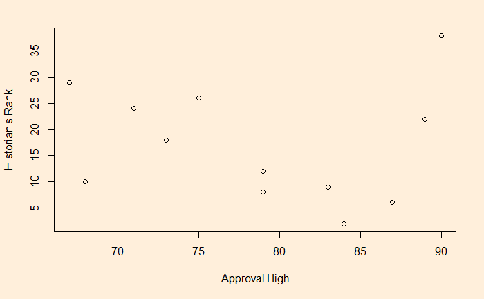
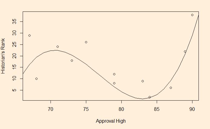
A usual tendency in regression is to chase better R-squared by increasing the dependent variables and ending up overfitting. Overfitting is a term used when your model is too complex that it sharts fitting noise. An example is this dataset taken from Regression Analysis Book by Jim Frost. It describes the highest approval ratings of the US presidents and their rank by historians.

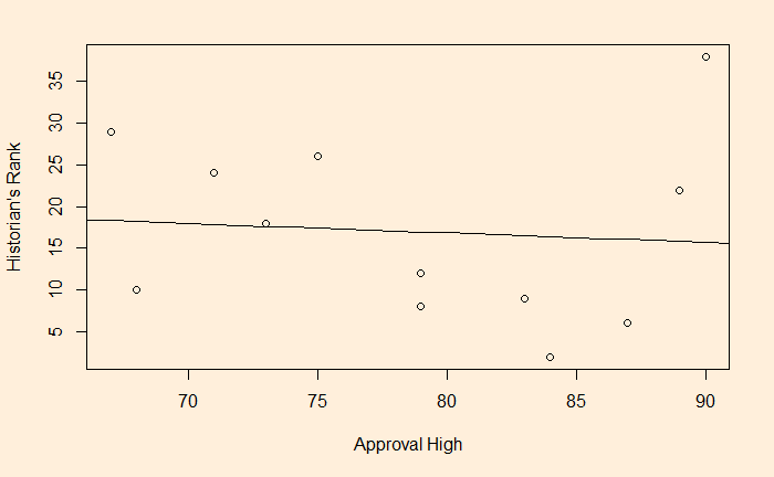
First, we try out linear regression and check the goodness of fit.

lm(Presi_Data$Historians.rank ~ Presi_Data$Approval.High)

The R-squared value is close to zero (0.006766). Now, we try cubic fit.

model <- lm(Presi_Data$Historians.rank ~ Presi_Data$Approval.High +  I(Presi_Data$Approval.High^2) + I(Presi_Data$Approval.High^3))

But with an impressive R-squared (0.6639)

Now, try thinking how one can explain this complex relationship, i.e. Historians Rank = -9811 + 388.9 x Approval High -5.098 x Approval High^2 + 0.02213 x Approval High^3!

Non-Linear Regression – Overfitting Read More »

Guys Finish Last

Do you remember the last time you were in a queue that reached the counter ahead of others who joined at similar times as you did? It could be a bit of a struggle to recollect, but I’m sure you remember the time you finished the last! Let’s analyse what must be happening with you.

Clue 1: Selective memory

The simplest explanation for your troubles is selective memory. Don’t you remember that day you wanted to write down a number in a phone call and found the pen was not working? You know it was not the first telephone you attended in life where you had to write something down. And you had a pen that worked, but you took it for granted – after all, the purpose of that device is to write.

You are more likely to recollect the days you finished last than you did first. And that is human nature. Biologists speculate this is part of an evolutionary defence mechanism that you remember the past incidents that led you to trouble, perhaps as a trigger not to repeat them.

Clue 2: Probability

We have seen several examples already. You are entering a billing section of a store that has ten lines. If you pick a random queue, what is the probability that you end up in the fastest? The answer is 1/10. To state it differently, what is the chance that you are not the fastest? Nine out of ten. Then you argue that it was not accidental and that you selected the shortest. There are two possible responses to that feeling.

First, all the others in the hall also (think they) selected the shortest, and your selection, regardless of how you felt, was still random. The second explanation concerns the specific information about your choice that you lacked and the others had. It was short as there was something in that queue – a slower attendant or people with items that required more time for the check-in. And you just took that. Once you are in the line and start measuring the average time taken by the others, you get into what is known as the inspection paradox.

Clue 3: WAITING-TIME PARADOX

We have seen it before in the name of the inspection paradox and waiting time paradox. We proved mathematically that the actual waiting time is longer than the theoretical average calculated based on the frequency of occurrences.

In short

Next time the feeling occurs on why it happened only to you and not anyone else, think again. It is more likely that the others, too, feel the same; after all, the “you” I chose in the description is just an arbitrary choice.

Reference

The formula for choosing the fastest queue: The conversation

Guys Finish Last Read More »

Football’s Double Poisson

It is world cup season. The world championship for football, or soccer to some, arguably one of the world’s most popular sports spectacles, is happening now in Qatar. On the eve of the start, the prestigious science journal, Nature, published an article on the importance of data science to football’s evolution to its current state.

At the end of the paper, the authors quote a prediction table based on a double Poisson model that predicted the 2020 European championship with reasonable accuracy.

Here, we “cherry-pick” one of the teams, Belgium, which failed to qualify for the knock-out stages, nonetheless the top-billed squad by the model and estimate the possibility of them qualifying from the preliminary stages.

The model estimate Belgium to have 13.88% of winning the cup, followed by Brazil at 13.51. So, we estimate that if Belgium reached the tournament’s final, it would have a 13.88/(13.88+13.51) = 50.7% chance of winning. Therefore,

The chance of winning the cup = probability of reaching the final (P1/2) x probability of winning the final.
P1/2 = 0.1388 / 0.507 = 0.27 (27%).

Extending the argument further, P1/4, the probability of Belgium in the semi-finals is, P1/4 = 0.27/(13.88/(13.88+11.52)) = 0.5.
P1/8 = 0.5/(13.88/(13.88+5.29))= 0.69.
P1/16 = 0.69/(13.88/(13.88+0.69)) = 0.72.

So, Belgium had a 28% chance of not qualifying for the playoffs, and it happened that way! Note that the chances, 11.52, 5.29 and 0.69, are taken from the same table as the winning chances of the 4th, 8th and 15th teams.

Making it broader

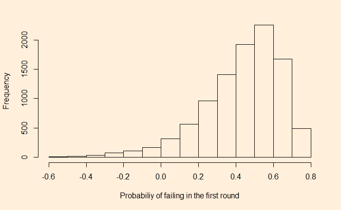
Here we have assumed that Belgium met Brazil (winning probability = 13.51), Argentina in the second (11.52%) etc. In reality, we don’t need to make such assumptions. Let’s consider an extreme case, which is also not possible as the qualifying teams go via a narrow path forward, where any team in the top 15 could meet Belgium in each round. We run a Monte Carlo with the following code.

nn <- 10000
  
sec_round <- replicate(nn, {
 round <- sample(c(0.1351, 0.1211, 0.1152, 0.0965, 0.0724, 0.0637, 0.0529, 0.0378, 0.0336, 0.0317, 0.0256, 0.0233, 0.0146, 0.0067), 4, replace = FALSE)

P_1 <- 0.1388
P_12 <- P_1/(P_1/(P_1+round[1]))

P_14 <- P_12/(P_1/(P_1+round[2]))

P_18 <- P_14/(P_1/(P_1+round[3]))

P_116 <- P_18/(P_1/(P_1+round[4]))

1 - P_116 
})

And the answer is in the following histogram.

I must say that the analysis is meant for fun, with hardly any speck of reality in it. Since the calculations are done in reverse, the conclusions don’t prove that a team with the highest (13.88%) chance to win the cup will go out from the first round with a 40% probability. On the contrary, it only states that even a team with only a 60% chance to reach the second round can still have a 13.88% chance to win!

Reference

How big data is transforming football: Nature
Double Poisson model for predicting football results: Plos One

Football’s Double Poisson Read More »

It’s All About the Fourth Quarter

Let’s turn our attention to NBA. This time, we will analyse a common belief – that the matches are decided in the fourth quarter. Apart from that, we will also try a bunch of other hypotheses, such as home-away advantage. We have collected the first 100 matches of the NBA season 2021-22 to test the hypothesis.

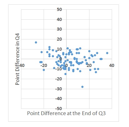
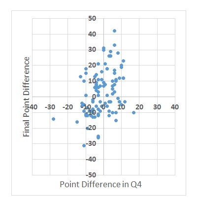
First, we check if there is any relationship between the point difference in the fourth quarter with what is at the end of the third.

The graph shows no real relationship. So, the fourth quarter is different; but do they determine the winner? That’s next.

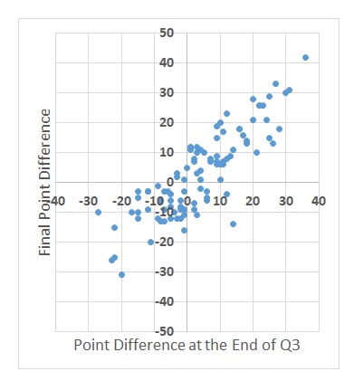
The correlation here also is modest. That brings us to the all-important graph – the winner vs the point difference at the end of the third quarter.

Winner till Q3 wins the match

The result is obvious. There seems a much better correlation between the leader until the third quarter to the ultimate winner.

It’s All About the Fourth Quarter Read More »

T. gondii Continues

The previous post that a parasite triggers wolves to become courageous leaders may sound fantastic, but something difficult to accept as a fact. If you recall rule number one of statistics: “correlations are not causations”, you may realise that there could be other explanations to understand wolves’ the peculiar behaviour of some wolves who happened to have been infected.

What if the same behaviour, aggression, tendencies to walk out of the pack, and courage is the reason that caused the disease in the first place? The claim is not entirely without reason, as the animal gets the illness from cougars that share the same land space. After all, these are observational studies. Naturally, we would have liked to see results from a controlled study.

The researchers selected 64 laboratory rats and infected 32 of them (experimental group) with a cyst-forming strain of the parasite. The other 32 are given a placebo (control group). The rates were exposed to an area, and its corners contained distinct odours, representing four species – rat, cat, rabbit and neutral.

Now, a bit of evolution. Small mammals under heavy predation pressure evolved as species that could identify and avoid the presence of their predators. For rats, it is the ability to smell and avoid cats. You know already that it is not a rat that decided to build the capability to help itself; rather, as per the principle of survival of the fittest, only those rat species survived and had multitudes of offspring. Studies have shown that rats don’t lose the anti-predator behaviour (aversion to cat smell) even after hundreds of generations without having felt the presence of a cat.

And this is where our study got interesting. In the experiment, the status of the rats, infected or otherwise, did not change their movement towards the three non-cat selling areas. Whereas the uninfected rate disproportionally avoided cat-smelling spots compared to the infected.

References

T. gondii Continues Read More »