July 2022

Monty Hall: Appreciating the Host

We have discussed the Monty Hall problem already a couple of times. One reason why people make this mistake is that they forget the role of the host in reducing the uncertainty of the car’s location. In other words, when the host eliminates one wrong door, he doubles the chances for the participant.

100 doors

Imagine a modified game in which there are 100 doors. You pick one. There can not be two opinions here that the chances of guessing the right door (having a car behind it) is one in one hundred. The host then opens all but one opening and shows you 98 goats. Will you switch this time? Or do you still think your original choice has a 50% probability of finding the car?

Monty Hall: Appreciating the Host Read More »

Error, Noise and Bias

We have built the definitions of data scatter (noise) and bias based on a group of data points in the previous post. This time, we estimate the mean squared errors of the data.

Noise

Here is a collection of data:

If you are not aware of the bias in the data, you would have calculated the error in the following way. Estimate the mean, calculate deviations for each of the points from the mean, square them and calculate the mean of the squares.

Note that this is also called the variance. For our data, the mean is 40, and the mean square ‘error’ is 15.75.

Somehow, you learned that the data was biased, and the true value was 45 instead of 40. Now you can estimate the mean square error as given below.

The value of this quantity is 39, which is the combined effect of the error due to noise and bias.

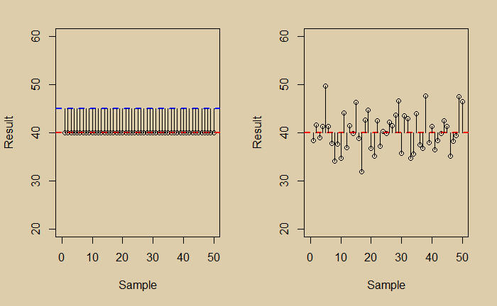
One way of understanding the total error is to combine the error at zero scatter and the error at zero bias. They are represented in the two plots below.

The mean squared error (MSE) in the zero-scatter (left) is 25 (square of the bias), and the zero bias is 15.75. And the sum is 40.75; not far from the total (39) estimated before.

Why MSE and not ME?

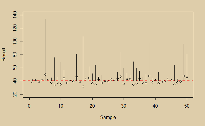
While you may question why the differences are squared, before averaging, it is apparent that in the absence of squaring, the scattered data around the mean, the plusses and minuses, can cancel each other and give a false image of an impressive data collection. On the other hand, the critics will naturally express their displeasure at seeing an exaggerated plot like the one below!

This is what happens when the errors are squared.

Reference

Noise: A Flaw in Human Judgment: Daniel Kahneman, Olivier Sibony, Cass R. Sunstein

Error, Noise and Bias Read More »

Variance and Bias – Continued

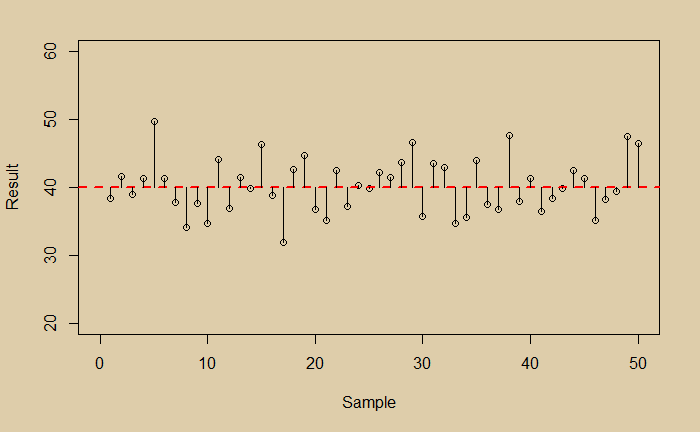
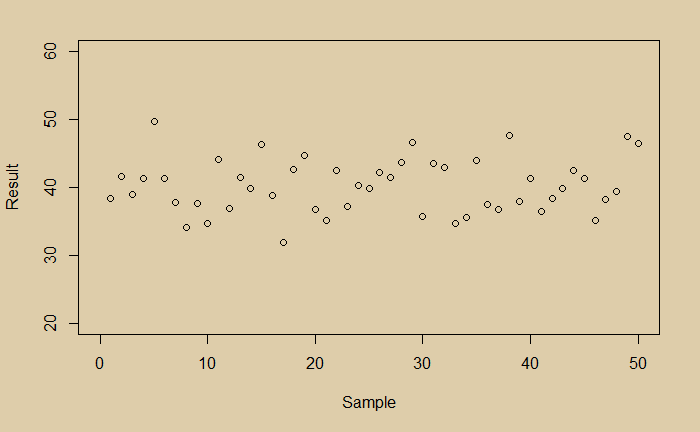
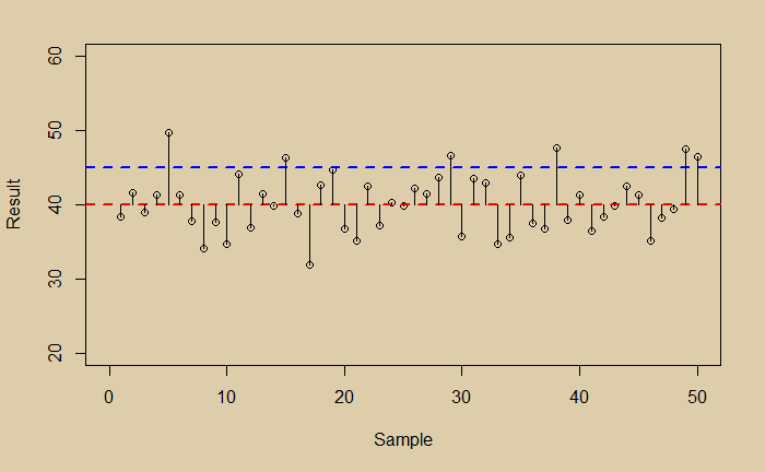
Imagine you did a measurement and collected the following 50 data points.

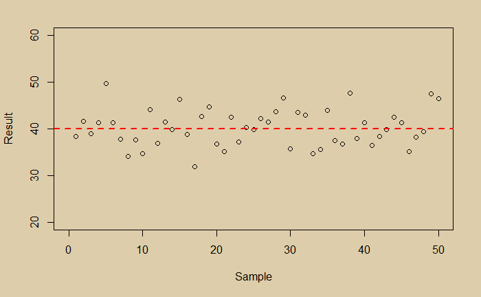
What would you conclude? You see a little noisy data. You do a regression and get the following average line.

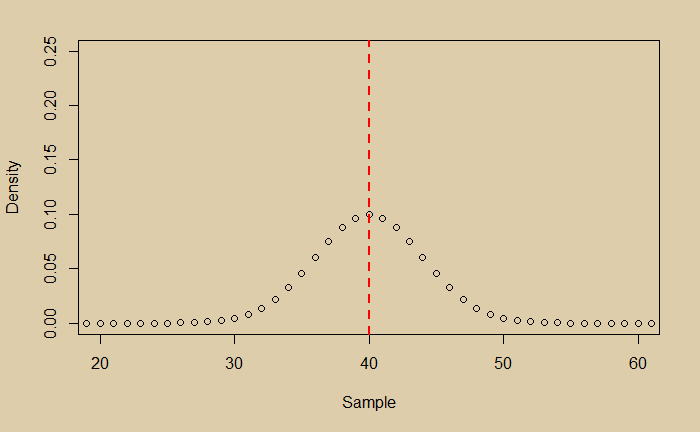
Now you are happy that you managed the random scatter of the data; you got the expected value of the experiment. And it is 40. You then plot the distribution of your data and find it is perfectly normal.

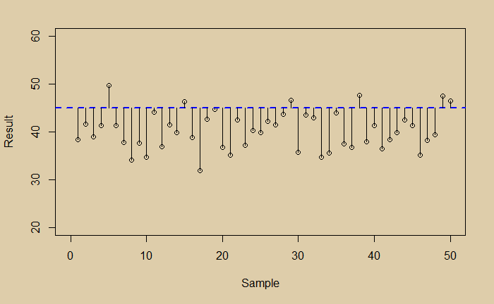
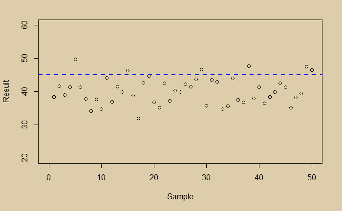
Imagine your true value is 45, and your experiment had a bias.

Suddenly you have two problems, scatter (noise) and bias. Which one is a bigger problem to address?

Variance and Bias – Continued Read More »

Variance and Bias

Mean

We know what the mean for the distribution of random variables is; it is called the expected value. You can calculate it by multiplying outcomes by their respective probabilities and sum over all those outcomes.

E[X] = \sum\limits_{i=1}^n (p(X_i)*X_i) = \mu

If the variables are discrete and all the probabilities are equal (equal weightage), add them up and divide by the number of variables.

\mu = \frac{1}{n}\sum\limits_{i=1}^n (X_i)

Variance

The spread of values around the mean is variance. It is calculated by calculating the mean of (expected value of) square of sample values after subtracting the mean.

E[(X - \mu)^2] = \sum\limits_{i=1}^n [p(X_i)*(X_i - \mu)^2]

Like in the earlier case, for an equally likely case (all p(Xi) are equal), variance can be calculated by adding all the squares and dividing by the total number.

Var(X) = E[(X - \mu)^2] = \frac{1}{n}\sum\limits_{i=1}^n [(X_i - \mu)^2]

Bias

So far, we have assumed unbiased samples (e.g. fair coin, fair dice etc.) in our discussions. In such cases, the true values equalled the expected values. It is not the case in real life, where biases do occur. Bias is the difference between the average value and true value. In other words, you get the true value after subtracting bias from the average of the estimators.

Bias(\hat\theta) = E[\hat\theta] - \theta

Variances and biases are two causes of error in data. How they are related or not related is the topic of another discussion.

Variance and Bias Read More »

Law of Large Numbers

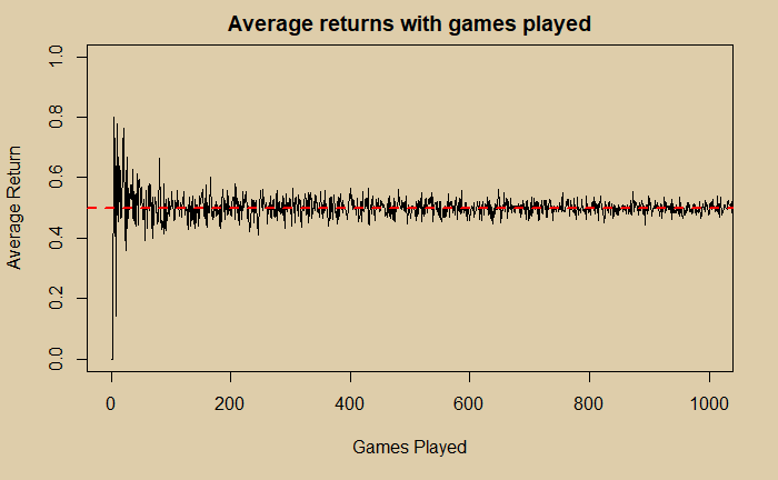
The last time we did random sampling and counting, also known as the Monte Carlo experiments. Today we build two programs to demonstrate what is called the law of large numbers through two examples, coin tossing and die rolling. In case you forgot, the law of large numbers is a phenomenon where the actual value starts converging to the expected value as the number of events increases.

Coin Toss

Imagine you are in a coin game: you get 1 dollar for a head and nothing for a tail. What is the average amount you are gaining from the play? We create an R program that calculates the average of several sampling outcomes and plots it as a function of the number of games played.

fin_number <- 1000
xx <- replicate(fin_number,0) # initiating vector
yy <- replicate(fin_number,0) # initiating vector

for (rep_trial in 1:fin_number) {
 
win_fr <- replicate(rep_trial, {
  try <- sample(c(1,0), size = 1, replace = TRUE, prob = c(0.5,0.5))
  })
 xx[rep_trial] <- rep_trial
 yy[rep_trial] <- mean(win_fr) 
}


par(bg = "#decdaa")
plot(xx,yy, type = "l", main = "Average returns with games played", xlab = "Games Played", ylab = "Average Return", xlim = c(0,1000), ylim = c(0,1))
abline(h = 0.5, col="red", lwd=2, lty=2)

The code uses four functions in R – for loop, replicate, sample and plot. The red dotted line represents the expected probability of 0.5 for a head in coin-tossing.

Dice Roll

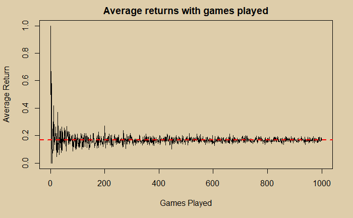
In this game, you get one point when you roll a 1, nothing otherwise.

fin_number <- 1000
xx <- replicate(fin_number,0)
yy <- replicate(fin_number,0)

for (rep_trial in 1:fin_number) {
 
win_fr <- replicate(rep_trial, {
  die_cast <- sample(c(1,2,3,4,5,6), size = 1, replace = TRUE, prob = c(1/6, 1/6, 1/6, 1/6, 1/6, 1/6))
if (die_cast == 1) {
  counter = 1
} else {
  counter = 0
}
  })

xx[rep_trial] <- rep_trial
yy[rep_trial] <- mean(win_fr) 

}

par(bg = "#decdaa")
plot(xx,yy, type = "l", main = "Average returns with games played", xlab = "Games Played", ylab = "Average Return", xlim = c(0,1000), ylim = c(0,1))
abline(h = 1/6, col="red", lwd=2, lty=2)

You know the probability of obtaining a 1 from the rolling of a fair die is (1/6), which is represented in the figure by the red dotted line.

The Roulette

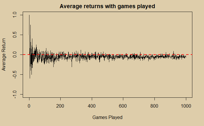
I can not stop this post without referring to Roulette. Here is what we obtain, by setting probabilities to (18/38) and (20/38) for winning 1 and -1, respectively.

fin_number <- 1000
xx <- replicate(fin_number,0)
yy <- replicate(fin_number,0)

for (rep_trial in 1:fin_number) {
 
win_fr <- replicate(rep_trial, {
  try <- sample(c(1,-1), size = 1, replace = TRUE, prob = c(18/38,20/38))
})
xx[rep_trial] <- rep_trial
yy[rep_trial] <- mean(win_fr) 
}

par(bg = "#decdaa")
plot(xx,yy, type = "l", main = "Average returns with games played", xlab = "Games Played", ylab = "Average Return", xlim = c(0,1000), ylim = c(-1,1))
abline(h = 0.0, col="red", lwd=2, lty=2)

You can see that you have more possibilities to get some money (> 0) as long as you leave early from gambling. As you keep playing more and more, your chances of making anything in the end diminish.

Law of Large Numbers Read More »

A Banana Problem and an R Solution

The last banana is a probability riddle by Leonardo Barichello that I found in a TedEd video. It is a thought experiment as follows:

Two players are playing a game by rolling two dice. If the higher number of the two is 1, 2, 3 or 4, player A wins, whereas if it is 5 or 6, player B wins. Who has a better chance of winning the game?

Let’s play a million times

The primary aim of this post is to develop an R code that generates a million such games and calculate how many times A and B win. We will then compare the results with the theoretical solution.

A die has six sides, and an unbiased one gives equal chances for each of its faces, numbered one to six. In other words, the probability of getting any of the numbers is one in six or (1/6). So, first, we need to create a die, roll it two times and get two random outcomes.

Random generator

The sample function in R can make random numbers from the given sample space at the specified probabilities.

sample(c(1,2,3,4,5,6), size = 2, replace = TRUE, prob = c(1/6, 1/6, 1/6, 1/6, 1/6, 1/6))

The code has four arguments: the first one, c(1, 2, 3, 4, 5, 6), is an array of all possible outcomes. The second is size, the number of times you want to choose. Here we gave two, corresponding to the two dice rolls. ‘replace is TRUE’ because you want to replace what came out in the first roll before the second roll. Finally, you provide probabilities of occurrence for each element in the sample space. There are six in total, and because it is a fair die, we give them equal chances (1/6). When I ran the code 5 times, the following is what I got.

[1] 1 6
[2] 1 4
[3] 2 3
[4] 4 6
[5] 2 6

If you recall the rules, player A wins two times (games 2 and 3), and player B wins three (games 1, 4 and 5). But, to get a reasonable certainty for the probability by counting the outcomes (the frequentist way), you need to play the game at least 1000 times! And we are going to automate that next.

Repeating the exercise

The replicate function can repeat an evaluation as many times as you specify. A simple example is.

replicate(3,"Thougthful")

can give an output

[1] "Thougthful" "Thougthful" "Thougthful"

Instead, if you want to give a chunk of calculations and repeat, you can use brackets like this:

jj <- replicate(3, {
          1
  })
jj

The output of the above expression is 1 1 1.

Back to bananas


repeat_game <- 1000000

win_perc_A <- replicate(repeat_game, {

   die_cast <- sample(c(1,2,3,4,5,6), size = 2, replace = TRUE, prob = c(1/6, 1/6, 1/6, 1/6, 1/6, 1/6))
     if (max(die_cast) <= 4) {
     counter = 1
   } else {
     counter = 0
   }

}
)

mean(win_perc_A)

The code will repeat the sampling a pair of numbers, estimate the maximum (max function) of the duo and count if the maximum is less than or equal to 4 (by assigning 1 for the target and 0 otherwise) a million times. Finally, you either count the successes (of A) or calculate the mean; I went for the latter.

To end

The analytical solution is rather easy. The criterion for player A to win this game is if both rolls remain at four or below. The probability of the first roll remaining at four or below is (4/6). The same is for the second roll. Since the rolls are independent, you get the joint probability of two die rolls by multiplying the numbers. (4/6) x (4/6) = 16/36 = 0.4444.

Now, what was the answer to the simulation? By taking an average of the counts of a million games, the answer was 0.444193. Not bad, eh?

So, the answer to the riddle? You better be player B in this game with about a 56% chance to win.

The last banana: A thought experiment in probability – Leonardo Barichello

A Banana Problem and an R Solution Read More »

Permutations and card Shuffle

Permutations enable us to calculate the number of ways of arranging something and when the order matters. An example is the number of unique manners of placing three people, A, B, and C, on a podium, where first, second and third matter!

A B CA C BB A C
B C AC A BC B A

The formula for the permutations of n available options taken r at a time is nPr.

_nP_r = \frac{n!}{(n-r)!} = \frac{3!}{0!} = 3 * 2 * 1= 6 \text{; for 0! = 1} \\

So, what is the number of unique ways of shuffling a deck of cards?

_{52}P_{52} = \frac{52!}{(52-52)!} = \frac{52!}{0!} = 52! = 8.1 \text{x}10^{67}

Eight followed by 67 zeroes is a mind-blowingly large number and is far more than the number of atoms on this planet. Next time, when you shuffle a deck of cards, remember this arrangement may never have happened in this history and may never be happening again.

Factorial Calculator

Number of atoms in the world: Fermilab

Permutations and card Shuffle Read More »

The 100 Prisoners Problem

In the previous post, we have seen a variation of the 100 prisoners problem applied to the Monty Hall problem. But what is the 100 prisoners problem?

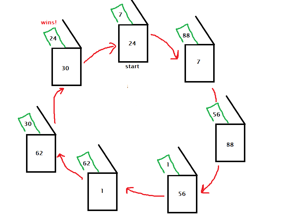
One hundred prisoners numbered 1 to 100 are given a choice to free themselves if they all find their numbers, written on a piece of paper, randomly kept inside 100 boxes numbered 1 to 100. In other words, the bit carrying number 8 could be inside box 64, #21 inside box 99 etc. The room that keeps the boxes allows only one prisoner at a time, and he can open a maximum of 50 boxes. Even if one fails in his attempt, the whole group loses, and none will walk free. Prisoners can discuss strategies only before the game.

The Strategy

Suppose each player tries opening boxes at random. The probability of a person finding his number from 100 boxes by opening 50 is (50/100) or (1/2). For 100 people to find their numbers, the chances are (1/2) multiplied 100 times or (1/2100), a number close to zero.

Instead, they decide on a strategy; the person first opens the box that carries his number. If he finds his number, fine or else he goes to the box that corresponds to the number inside the first box. It continues until one of the two things happens. He finds his number, or he reaches the maximum of 50 attempts. This strategy can raise the probability of success to a mind-boggling 31%!

To understand this, take the case wherein the prisoner finds his number inside a box. If he continues the strategy, the number he just discovered, which is his number, will lead to the container that carries his number, which is nothing but the first one he opened. Or he always completes a circle of 50 (or lower) boxes if he is successful. Every unsuccessful attempt means the (unfinished) loops are longer than 50.

The travel of prisoner number 24

Each prisoner makes one loop

So the problem becomes the collection of such loops. The probability that such a cluster has no loop larger than 50 is 31%.

The 100 Prisoners Problem Read More »

Car – Key Challenge

Here is a variation of the Monty Hall problem based on the 100 prisoner challenge.
Three objects – a car, a key and a goat – are randomly placed behind three doors. You play the game with a partner. And each of you can open a maximum of two doors, one person at a time. In order to win the car, the first player must find the car, and the second the key.

If the players play at random, the probability of the first player to find the car in two attempts (out of the possible three doors) is 2/3. Similarly, for the second, finding the key is 2/3. The probability of winning is (2/3) x (2/3) = 4/9 = 44.4%.

Strategy

If they do the following strategy, they can maximise the probability to (2/3), which is equal to the chance of any of them reaching their individual goal. Here is how they do it.

Person 1 goes and opens door 1. If she finds the car, she completes her task and over to person 2. If instead, she finds a key, she will try door 2. Whereas, if she finds a goat on the first attempt, she will go for door 3.

The second person might not start 1 out of 3 times, i.e. whenever the first person was unsuccessful. If that is not, she will first open door 2. If it was a key, the team wins. If she finds a goat behind door 2, she will open door 3; if it is a car, she will open door 1. The possibilities are in the table below.

Sequencecar-key-goatcar-goat-keykey-car-goat
Player 1door 1: cardoor 1: cardoor 1: key
door 2: car
Player 2door 2: key
(wins)
door 2: goat
door 3: key
(wins)
door 2: car
door 1: key
(wins)
Sequencekey-goat-cargoat-key-cargoat-car-key
Player 1door 1: key
door 2: goat
door 1: goat
door 3: car
door 1: goat
door 3: key
Player 2no gamedoor 2: key
(wins)
no game

You can see that whenever the first person does her job (wins the car), the second one gets the keys.

Car – Key Challenge Read More »

The St. Petersburg Paradox

We know what the expected value theory is. The St. Petersburg paradox seriously challenges that. It is a coin-tossing game and it goes like this:

A casino makes a coin-tossing game for a single player. In the first toss, if you get a head, you win a dollar, and the game ends. If it’s a tail, the game continues but doubles the payoff (two dollars) for the next round. At the appearance of the first head, you go home collecting whatever you won. What is the price you want to pay to the casino to enter the game?

The expected value

Let’s see what the expected value of the game is.
EV = P(1 T) x V(1 T) + P(2 T) x V(2 T) + P(3 T) x V(3 T) + …
where P(1 T) is the probability of one tail and V(1 T) is the value of one tail etc.
EV = (1/2) x 2 + (1/4) x 4 + (1/8) x 8 + …
= 1 + 1 + 1 + 1 … = Infinity.

Therefore, the rational player must be willing to pay any price to get into the game!

In reality, you will not pay that amount. Think about this: what is the probability of getting a head in the first toss (and you get one dollar)? It is 50%. Similarly, the chance of ending up with 4 dollars is 25%, and so on.

This disparity between the expected value and the reality is the St. Petersburg paradox.

Bernoulli’s solution

Daniel Bernoulli suggested using utility instead of value to solve this problem. The utility is a subjective internal measure of the player towards the gain from the game. According to him, the utility of the additional amount (earned from the contest) was a logarithmic function of the money.

u(w) = k log(w), w represents the wealth. It is logarithmic, he hypothesised, as there is an inverse relation (1/w) between change in wealth and its value. Mathematically,
du(w)/dw = 1/w

With this information, let’s rework the expected utility of this game

nP( nT)wu(w)
u = logw
(k = 1)
Expected
Utility
11/220.690.35
21/441.390.35
31/882.080.26
51/32323.470.11
101/102410246.930.007
1.07

Unlike the previous case, the sum of utilities converges.

The St. Petersburg Paradox Read More »