February 2022

Elusive Justice

We have seen perceived culpability vs probability distribution of evidence and their overlapping nature in the last post. It offers a simple picture, but the message demonstrates the difficulties of establishing justice for all. Today, we will go a step deeper by invoking signal detection theory, a strategy that can help detect signals from noise.

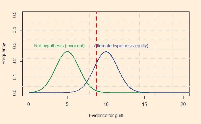
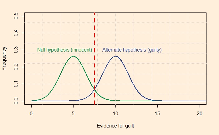
One technique to raise the level of justice (reduce misses and false alarms) is to increase the distance between the distribution curves from each other. Let’s look at it quantitatively: imagine you want not more than 5% misses and 5% false alarms, then the separation required between the two curves should be something like the following picture.
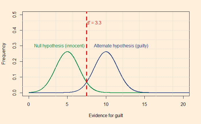
The red dotted line passes through the point on the 95th quantile of the green curve (calculated by the R formula, qnorm(0.95, 5, 1.52), where five is the mean and 1.52 is the standard deviation). You already know the meaning of 95% – it is 1.64 standard deviations away from the mean (equivalent to the one-sided confidence interval). The line also should match the left 5% of the blue curve (qnorm(0.05, 10, 1.52). One way to quantify the separation is to estimate the distance between the two distributions as a function of the standard deviation of the innocent.

d' = \frac{\mu_g - \mu_i}{\sigma_i} \\ \\ \mu_g \text{ = mean of guilty, }\mu_i \text{ = mean of innocent, and } \sigma_i \text{ = standard deviaton of innocent}

For the above plot, the separation is 3.3 standard deviations. If you wanted to see a more just system with a maximum of 1% errors, you need a detachment of 4.7.
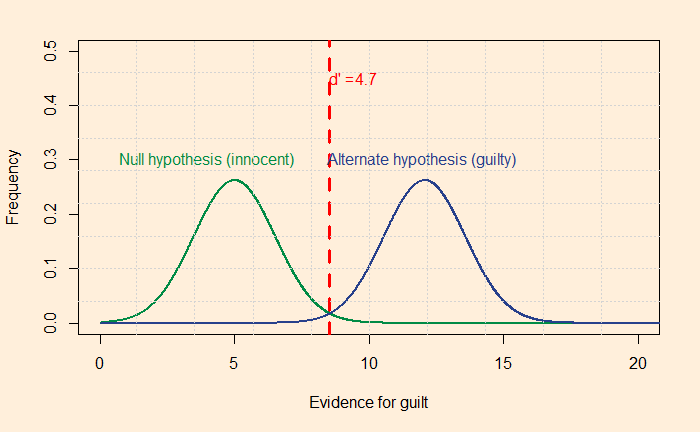
Are 3.3 and 4.7 realistic?

Unfortunately, the answer is no! Look at some indicators that experimentalists have found out. For spotting lie, the d’ values obtained by studies stand at 0! d’ ranged from 0.6 to 0.9 for the polygraph test; the best-in-class gave close to 2.5, but that was exceptional.

Then come eyewitnesses: researchers did a meta-analysis of 120 studies and found d’ values of 0.8 on facial identification. Following is how d’ = 0.8 appears.
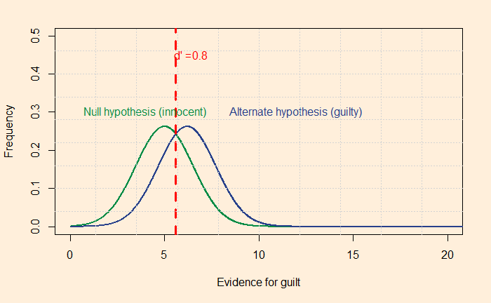
Medical tests have typically higher levels of d’ values but fall short of 3 (CT scans 3.0, mammograms 1.3 etc.), suggesting getting a 5% error level is a target difficult to achieve. What more can we do? We will see next.

Do juries meet our expectations?: Arkes and Mellers

Rationality: Steven Pinker
Elusive Justice Read More »

Justice for All

We all like to see justice happening in every trial. What is justice? In simple language, it is the conviction of the guilty and the acquittal of the innocent. In the court, jurors encounter facts, testimonies, arguments in support and against the defendant. The number and variety of evidence make them feel like random, independent events and make the hypothesis (that the accused is guilty or not) in front of the judge a distribution!

Overlapping Evidence

To illustrate the complexity of decision making, see the following two distributions (I chose uniform distribution as an example).

You can imagine four possibilities formed by such overlapping curves. The right-hand side tail of the innocent line (green) that enters the guilty (blue) region leads to the conviction of the innocent. The opposite – acquittal of the guilty – happens for the left-hand side tail of the guilty line that enters the non-guilty. The dotted line at the crossover of the two curves represents the default position of the decision or the point of optimal justice. At that junction, there are equal frequencies for false alarms and misses.

10 guilty for 1 innocent

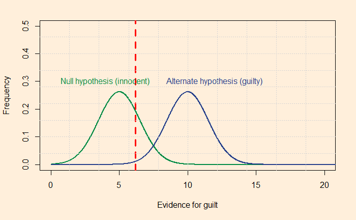
If the judge believes in Blackstone’s formulation, she will move her position to the right, as in the following plot.

The jury is willing to miss more guilty but assure fewer innocents are convicted. The opposite will happen if there is a zero-tolerance policy for the guilty; the examples in the real world are many, especially when it comes to crimes against national interest.

Errors and mitigations

So, what can jurors do to reduce the number of errors? We will look at more theoretical treatments and suggestions in the next post.

Do juries meet our expectations?: Arkes and Mellers

Justice for All Read More »

Binomial-Beta

Shaquille’s story continues. Last time, we made assumptions about each other’s feelings (hypotheses is the polished word!) for Shaq’s chance to enter the White House. Those assumptions were arbitrary: 0.9 and 0.2 for the probability of success or p. What about other factions? There are infinite of them between 0 and 1. This time, we will make no assumptions and take as many as possible using a continuous hypothesis generator.

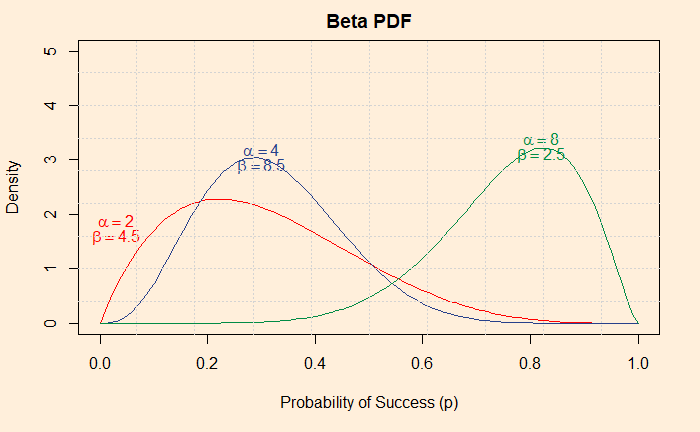
For that purpose, we will use the beta distribution function. Why beta? There is a reason for that, but we will know only towards the end. For now, we focus on what it can do for us more than what beta is. The beta distribution function can give a wide variety of probabilities for the entire range of p values. See three typical types (beta pdf uses two characteristic parameters, alpha and beta):

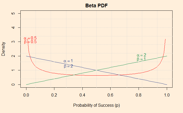
And three variety types:

The first reason to choose the beta distribution function (don’t get confused; this is not a beta function, which is a different beast) is that it takes the range of hypotheses (p) we are after as its input. i.e. 0 to 1.

What should Shaq and his friend choose?

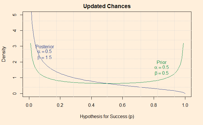
Remember, Shaq and his friend have strong views about getting inside the White House, and they are betting! So, which shape of the beta distribution function should they choose? They are unlikely to use more consensus-driven types, the curves that bulge in the middle. Who will bet when two opinions are towards a single idea? So, they chose alpha = 0.5 and beta = 0.5 as their prior hypothesis.

Bayes’s to help after the misadventure

We know what happened: Shaq failed to get inside without the prior appointment, so the outcome was zero success in the first attempt. Now, we predict what happens if he tries again (without actually doing and finding it). That is where Bayesian inference comes in handy. That is also the second reason for choosing the beta distribution function. Write down the Bayes’ rule here, i.e. posterior = likelihood x prior / sum of all possibilities. In the world of continuous functions, integrations replace additions.

\\ beta(\alpha_{posterior}, \beta_{posterior} | data) = \frac{likelihood * beta(\alpha_{prior}, \beta_{prior}) }{\int likelihood * beta(\alpha_{prior}, \beta_{prior})} \\ \\ \text{likelihood is binomial distribution function, as seen in the previous post} \\\\ \text{likelihood} = f(s; n,p) = \binom{n}{s} p^s (1-p)^{n-s}

Then a miracle happens: a complicated equation applied over the prior beta function results in a posterior beta function with a few minor modifications. The posterior is:

\\ beta(\alpha_{posterior}, \beta_{posterior}) = beta(\alpha_{prior + s}, \beta_{prior + n - s}) \\ \\ \text{in the present case} \\ \\ beta(\alpha_{prior}, \beta_{prior}) = beta(0.5,0.5) \\ \\ beta(\alpha_{posterior}, \beta_{posterior}) = beta(0.5 + 0, 0.5 + 1 -0 ) = beta(0.5, 1.5) \\ \\

New betting scheme

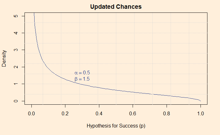
You know why s was zero and n was one, because Shaq did one (n) attempt and failed (s)! How does the new scenario, beta(0.5, 1.5), look? Here is the shape of beta(0.5, 1.5):

Putting together

The updated chance of Shaq getting inside the White House has come down after the information that he failed in his first attempt came out.

Shaq Denied Entrance: Washington Post

Bayesian Statistics for Beginners: Donovan and Mickey

Binomial-Beta Read More »

Shaq Goes to the White House

Shaquille O’Neil, popularly known as Shaq, is a basketball player and four-time NBA champion. He once had a bet with his friend about getting into the White House without prior permission. The wager was 1000 push-ups.

What is the chance of Shaq to be successful?

We can use binomial probability mass function (PMF) to estimate Shaq’s chance.

f(s; n,p) = \binom{n}{s} p^s (1-p)^{n-s}

Where n is the number of trials, s is the number of successes, and p is the probability of success.

Since Shaq was confident to bet, one can imagine that he would have given a higher value of p (say 0.9) for himself, whereas his friend would think lower (say, 0.2). If Shaq has one chance to show up, called a Bernoulli trial, associated probabilities with those two conditions are:

\\ f(1; 1,0.9) = \binom{1}{1} 0.9^1 (1-0.9)^{1-1} = 0.9 \text { and} \\ \\    f(1; 1,0.2) = \binom{1}{1} 0.2^1 (1-0.2)^{1-1} = 0.2

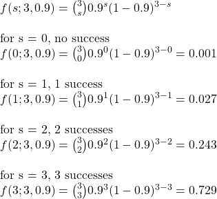
If Shaq makes three attempts, as per his view, the success rates are:

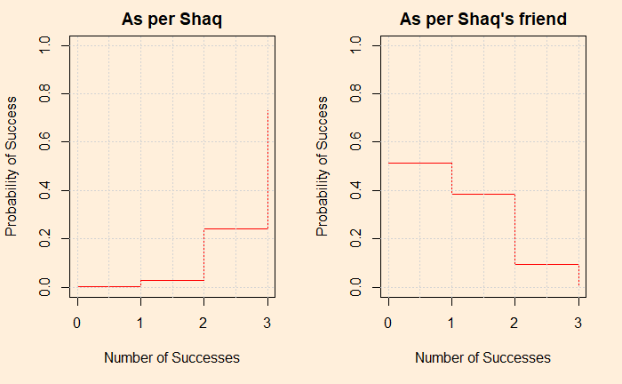
\\ f(s; 3,0.9) = \binom{3}{s} 0.9^s (1-0.9)^{3-s} \\ \\ \text{for s = 0, no success} \\ f(0; 3,0.9) = \binom{3}{0} 0.9^0 (1-0.9)^{3-0} = 0.001 \\ \\ \text{for s = 1, 1 success} \\ f(1; 3,0.9) = \binom{3}{1} 0.9^1 (1-0.9)^{3-1} = 0.027 \\ \\ \text{for s = 2, 2 successes} \\ f(2; 3,0.9) = \binom{3}{2} 0.9^2 (1-0.9)^{3-2} = 0.243 \\ \\ \text{for s = 3, 3 successes} \\ f(3; 3,0.9) = \binom{3}{3} 0.9^3 (1-0.9)^{3-3} = 0.729

The probability densities for Shaq and his friend, in graphical format, are:

Was Shaq successful?

No, he was not. He tried once but was stopped at the gate by the security! What would have happened had he made another attempt? More about that story and the use of Baysian in the next post.

Shaq Denied Entrance: Washington Post

Shaq Goes to the White House Read More »

Has UK Weathered the Storm?

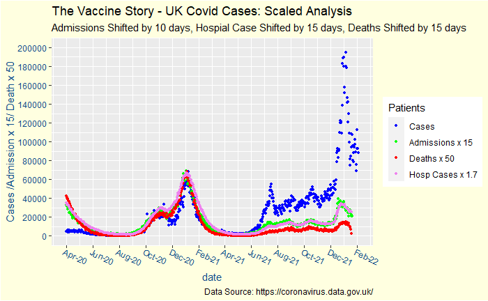
This post follows up on the one made in December. Covid’s latest variant, the omicron, was a storm that played havoc over the world. The actual calamity is not known yet, but there is a widespread feeling that it was milder.

The UK, one of the countries that captured and shared covid data from day 1, provides answers to some of those questions. Here is an update of what happened since last time. Note the deaths of the last few days are incomplete.

Critical parameters such as hospitalisations and deaths have been rescaled – both x and y axes – to coincide with the reported cases before the vaccine.

Has UK Weathered the Storm? Read More »

Who Wrote paper No. 54?

The Federalist papers were published anonymously in 1787-88 by Alexander Hamilton, John Jay and James Madison. Of the 77 essays, it is generally agreed that Jay wrote 5, Hamilton 43 and Madison 14. The remaining papers are either jointly written by Hamilton and Madison or by one of the two (not Jay). The problem was solved by Mosteller and Wallace using the Bayesian approach but using Poisson distribution.

We try to go through their approach using a simple Bayes’ rule. Consider paper no. 54. The starting point was the style of writing. Both Hamilton and Madison used similar styles, so it was difficult to get an answer that easily. The authors then looked for the usage of specific words, such as by, from, to, while, whilst, war etc. We take one such word, upon. The frequency distribution of upon collected from a set of papers published by Hamiton and Madison (including the ones outside The Federalist) is given below

Rate / 1000HM
0041
(0,1]17
(1,2]102
(2,3]11
(3,4]11
(4,5]10
(5,6]3
(6,7]1
(7,8]1
Total4850

Bayesian Problem

Let’s the formula the problem using upon as the tag word:
In paper 54, the word upon comes 2 times in the text (in 2004 words). So upon frequency is 0.99.
P(Hamilton|upon = 0.99) = P(upon = 0.99|Hamilton) * P(Hamilton) / [P(upon = 0.99|Hamilton) * (Hamilton) + P(upon = 0.99|Madison) * P(Madison)]

P(upon = 0.99|Hamilton) = (1/48) based on the frequency table
P(upon = 0.99|Madison) = (7/50) based on the frequency table
P(Hamilton) = can be 43/77 based on the existing known data of authorship. But we take 0.5
P(Madison) = can be 14/77 based on the existing known data of authorship. But we take 0.5

P(Hamilton|upon = 0.99 ) = (1/48 * 0.5)/(1/48 * 0.5 + 7/50*0.5) = 0.13 or 13%. Naturally, P(Madison|upon = 0.99) = 1 – P(Hamilton|upon = 0.99) = 87%

The Federalist Papers: No. 54

Inference in an Authorship Problem: Mosteller and Wallance, Journal of American Statistical Association, 58 (302), 275-309

Who Wrote paper No. 54? Read More »

Back to basics

In the beginning, there was dice

Probability on the margins

dice, game, random-1963300.jpg

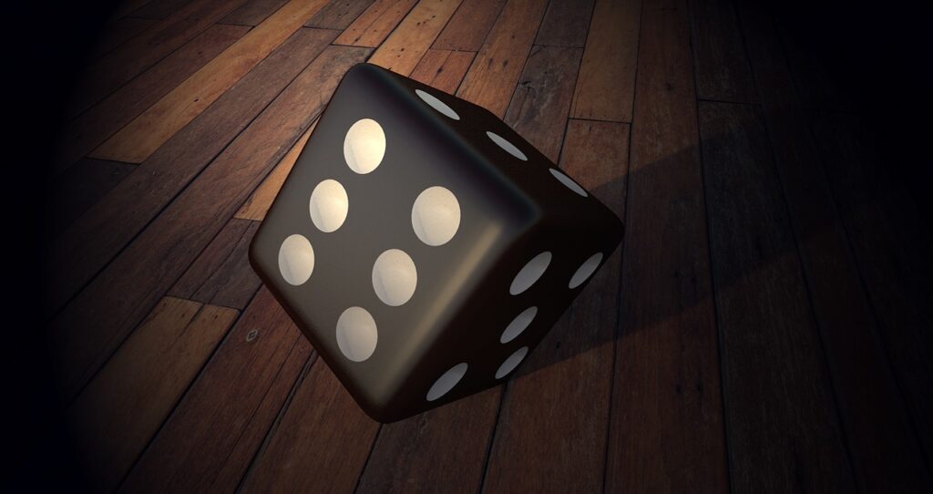
What is the probability of getting a 3 on a single roll of dice? You can calculate that by dividing the number of 3s by all possible numbers the die has.

123456

It is one 3 out of the possible six numbers, or (1/6). The probability of this type is called a marginal probability. The probability of one character of interest, say P(A). Or the one that is on the margins!

Two things at once

dice, die, cube-149215.jpg

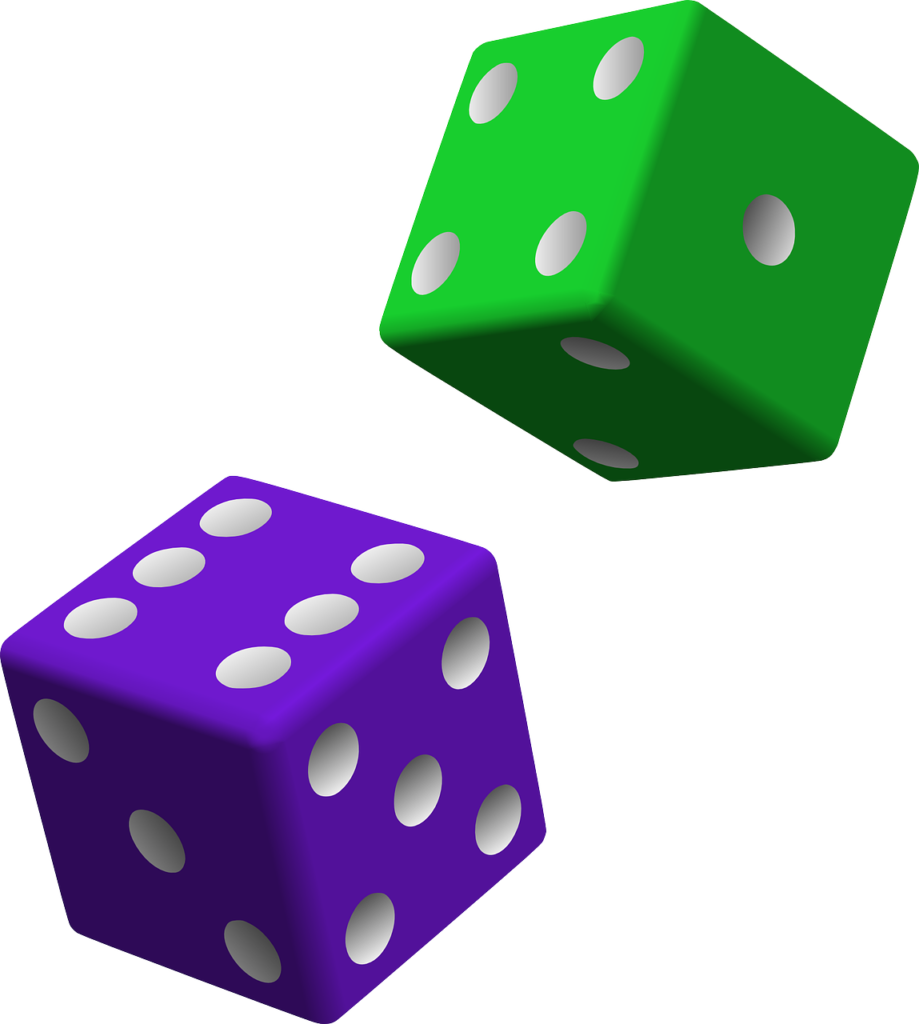
You throw two dice – one green and one violet. What is the probability that you get a green 3? It is the joint probability of two outcomes – a colour and a number – at once. The notation is:

P(Green \displaystyle \cap 3)

The upside-down U is the symbol of intersection or AND.

Green 1Green 2Green 3Green 4Green 5Green 6
Violet 1Violet 2Violet 3Violet 4Violet 5Violet 6

Only one instance of Green 3 in a total of possible 12 outcomes, so the joint probability is (1/12). When you hear joint, imagine an upside-down U and think it meant AND. What about the opposite?

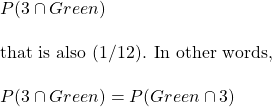
\\ P(3 \displaystyle \cap Green)  \\ \\ \text{that is also (1/12). In other words,} \\ \\ P(3 \displaystyle \cap Green)  = P(Green \displaystyle \cap 3)

Two things, with a clue

Now, what is the probability of seeing a 3 given it is a Green? This is a conditional probability and is represented as:

P(3 | Green)

You don’t need another table to answer that. If green is known, then there is only 1 out of 6 chances for a 3 or (1/6). What about the opposite, P(Green|3)? It’s (1/2) because if 3 is known, the choices are only two: green or violet. So, remember, P(A|B) and P(B|A) are not equal.

Formalising

We will start with the definition of joint probability as we had seen in AND rule earlier.

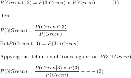
\\ P(Green \displaystyle \cap 3) =P(3 | Green) \text{ x }  P(Green)  --- (1) \\ \\ \text{   OR} \\ \\ P(3 | Green) = \frac{P(Green \displaystyle \cap 3)}{P(Green)}   \\ \\ \text{But} P(Green \displaystyle \cap 3) = P(3 \displaystyle \cap Green) \\ \\  \text{Appying the definition of}  \displaystyle \cap \text{once again: on } P(3 \displaystyle \cap Green) \\ \\ P(3 | Green) =  \frac{P(Green| 3) \text{ x } P(3)}{P(Green)}   --- (2)

Does the last equation remind you of something? Yes, it is one form of Bayes’ equation.

Let’s verify with numbers: first, equation (1) P(Green AND 3) = P(3|Green) x P(Green) = (1/6)x(1/2) = (1/12). Equation (2) P(3|Green) = P(Green|3) x P(3)/ P(Green) = (1/2) x (1/6) / (1/2) = (1/6).

The dice example is simplistic because the descriptors Green and 3 are independent. It’s fun once we have more dependent probabilities. But then, we have seen many of them in the previous posts.

Bayes’ equation

Look at the equation again.

P(3 | Green) =  \frac{P(Green| 3) \text{ x } P(3)}{P(Green)}

  1. The equation relates P(3|Green) with P(Green|3)
  2. The equation calculates P(3) from a known value of P(3)! Don’t you see P(3) on both sides? In case you don’t, P(3|Green) is, after all, P(3). The difference is that some additional information in the name of green is available to use. It is still about P(3) and not about P(Green). So to rephrase observation 2, the Bayes’ equation updates the knowledge of P(3) using additional information. That additional information comes from P(Green).

Back to basics Read More »

The Probability of 100 posts

Reaching one hundred days is a milestone. The general focus of my posts over these days, and also likely in the near future, has been about understanding risks, differentiating them from perceived risks and making decisions in situations of uncertainty using prior information, also known as Bayesian thinking. It started from the misery of seeing how the responsible agents of society -journalists, the political leadership, or whoever influences the public – ignore critical thinking and present a distorted view of reality.

Probability and evolution

A subplot that is closely associated with probability and randomness is the topic of evolutionary biology. It is hard to comprehend, yet the truth about life is that it moved from one juncture to another through chance. Evolution is misleading if you view the probability from hindsight. Changes happen through random errors, but one at a time, so that every step in the process is a high-probability event. Indeed, getting an error at a specified location during the body’s 30 trillion cell divisions is close to zero, but getting one at an unspecified somewhere is close to one. In other words, the designer has deeper trouble explaining a move than a drunken gambler!

Biases and fallacies

Next up is our biases and fallacies. The title of this post already suggests two of them – survivorship bias and the fallacy of hindsight. The probability of delivering an uninterrupted string of 100 articles in 100 days is small, and I would never have chosen the present title had I missed a post on one of these days. Now that it happened (luck, effort or something else), I claim I’ve accomplished a low-probability event. As long as I have the power to change the blog title until the last minute, I am fine. But scheduling a post today, for 100 days from now, with a caption of 200 days, is risky and, therefore, not a wise thing to do if you are risk-averse.

Deteminism or probability

Why does the subject of probability matter so much when we can understand physical processes in a deterministic sense? We grew up in a deterministic world, i.e. a world that taught us about actions and reactions, causes and effects. However, we also deal with situations where the outcomes are uncertain, which is the realm of probability. The impact of lifestyle on health, growth of wealth in the market, action of viruses on people with varying levels of immunity, the possibility of earthquakes, droughts, the list is endless. You can argue that the complexity of variables and the gaps in the understanding demand stochastic reasoning.

Updation of knowledge and Bayesian thinking

However imperfect it may be, Bayesian thinking is second nature to us. You are watching an NBA match in the last seconds, and your team is trailing by a point. Your team gets two free throws. What is in your mind when Steph Curry comes in for those? Contrast that with Ben Simmons. It is intuitive Bayesian thinking. It is not a surprise that you are more at ease with Curry’s 91% success rate in free throws than Ben, who is at 60%. You may not remember those numbers, but you know it from gut feeling.

Yet, being rational requires constant training. Your innate Baysian is too vulnerable to biases and fallacies. You start missing the base rates, confuse the hypothesis given the evidence with evidence given the hypothesis, or overestimate the prior due to recency bias. Surviving the sea of probability is hard, fighting the wind of lies and the sirens of misinformation. So what do you prefer, put wax in the ears, tie tight to the mast or get the rational power, listen to the music, and persist the voyage?

The Probability of 100 posts Read More »