This one is going to be one heck of a post, so hold tight. We need to start with the central limit theorem, and you know it by now. It says that the distributions of some properties of surveys, such as sum or average, follow a normal distribution if the sampling is proper. Go to this post for a refresher. By the way, don’t you think that if the sum is a distribution, the ‘average’ is also a distribution? After all, the average is the sum over a constant, the number of members in a survey.
Let me list down a few things in preparation for the upcoming roller-coaster ride.
- Population – everything; if you go and survey everybody, you don’t need anything else, end of the story. A country’s voting is done by all its population. The outcome has no uncertainty.
- Sample – sub-set of the population; all your statistics wizardry is required on samples. An opinion poll is on a selected sample, a few potential voters, so there is uncertainty.
- Mean – the average of measurements. The sample mean is what we get from each survey; finding the population mean is our task.
- Standard Deviation – a mathematical way of getting the variation of data. Use sample or population as add-ons, as before.
- Then, there are five notations: sample size is n, the population mean is mu (μ), the population standard deviation is sigma (σ), the sample mean is Xbar (X̄), and the sample standard deviation is S.
- Your task is to get μ and σ using one or a set of X̄ and S. All you have with you is trust in the Central Limit Theorem that says the mean of the entire distribution of all X̄ values is μ, and the standard deviation of the distribution of X̄ is σ/√n.
Mathematical Manipulations
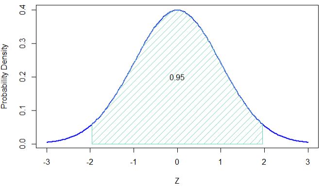
We know that X̄ shows a normal distribution (CLT). If you subtract a constant, the outcome is still a normal distribution. So we minus μ (we don’t know μ, but that doesn’t matter). Similarly, if you divide with a constant, the distribution is still normal, so we divide with σ/√n. The new distribution is uniform, but everything else has changed now. The new mean is 0 (remember: the mean of all survey results plotted as a distribution will coincide with the population mean). And the new standard deviation is 1 (because we divided it by the exact quantity). This distribution is known by a different name – the standard normal distribution, N (of the new variable Z).

Z forms a new normal distribution with mean = 0 and standard deviation = 1. Or N(0,1)
If That Holds
The probability that Z lies between -1.96 and +1.96 is 0.95, or 95%. If it were a normal distribution and we wanted to cover a distance of 2 times the standard deviation, shouldn’t it be plus or minus 2 and not 1.96? How did that happen? The answer is that we did not go for 2 sigma but a 95% interval. If you draw the standard normal distribution curve and check it, you will find that 95% of the distribution lies between -1.96 and +1.96.

Steps to Calculate Confidence Interval
Take the story in the previous post:
1 . Take the number of samples, n. n = 100
2. Calculate the mean of the sample, X̄. X̄ = 5
3. If you know the population standard deviation, σ. σ = 2. Divide σ with √n = 2 / √100 = 2 / 10 = 0.2. If you don’t know σ, you have to use S, the sample standard deviation. Assume S is also 2, and you get S /√n = 0.2.
4. If you know the population standard deviation, Choose the confidence interval. In our case, it was 95%. So as per the previous section, it is -(1.96 x 0.2) and +(1.96 x 0.2). That is 5 – 0.392 and 5 + 0.392 or [4.96, 5.4], which is my 95% confidence interval.
Not Over Yet
5. If you do not know the population standard deviation, As before, choose the confidence interval, which is 95%. The new interval is not between +(1.96) and -(1.96) but on a modified range. The value 1.96 becomes a function of the sample size -1 (the degrees of freedom). For smaller sample sizes, the number increases. For n = 2, it can be as large as +/- 12.71! In short, it is no longer a standard normal distribution but a t-distribution.
But we are lucky as our n is 100 (and the degrees of freedom = 99), and the multiplication factor is 1.984. -(1.984 x 0.2) and +(1.984 x 0.2). That is 5 – 0.3968 and 5 + 0.3968 or [4.96, 5.4], which is my 95% confidence interval.
Online T-distribution Calculator

