Alan knows the average fuel bill of families in his town last year was $260, which followed a normal distribution with a standard deviation of $50. He estimated this year’s value to be $278.3 by sampling 20 people. He then rejected last year’s average (the null hypothesis) in favour of an alternate of average > $260.
1. What is the probability that he wrongly rejected the Null hypothesis?
The probability is estimated by transforming the normal distribution with mean = 260 and standard deviation = 50 to a standard normal distribution (Z):

The ‘pnormGC’ function of the ‘tigerstats’ package makes it easy to depict the distribution and the region of importance.
library(tigerstats)

sample <- 20
null_mean <- 260
ssd <- 50
data <- 278.3

zz <- round((data - null_mean)/(ssd/sqrt(sample)), 2)
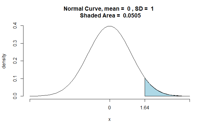
pnormGC(zz, region="above", mean=0, sd=1, graph=TRUE)
The probability of incorrectly rejecting the null hypothesis is 0.0505 (5.05%). It is the probability of Alan committing a Type I error.
If Alan accepts a 5% Type I error, he will reject the null hypothesis for every value > 278.3 and accept all values < 278.3.
2. If so, what is the probability of wrongly rejecting the alternate hypothesis that the true population mean for this year = $290?
sample <- 20
alt_mean <- 290
ssd <- 50
data <- 278.3

zz1 <- round((data - alt_mean)/(ssd/sqrt(sample)), 2)
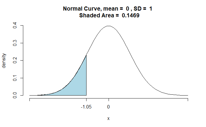
pnormGC(zz1, region="below", mean=0, sd=1, graph=TRUE)
The shaded area represents all the values < 278.3. And it is the probability of Type II error.

